Efficient Net
- Related Project: Private
- Category: Paper Review
- Date: 2024-01-15
EfficientNet: Rethinking Model Scaling for Convolutional Neural Networks
- url: https://arxiv.org/abs/1905.11946
- pdf: https://arxiv.org/pdf/1905.11946
- abstract: Convolutional Neural Networks (ConvNets) are commonly developed at a fixed resource budget, and then scaled up for better accuracy if more resources are available. In this paper, we systematically study model scaling and identify that carefully balancing network depth, width, and resolution can lead to better performance. Based on this observation, we propose a new scaling method that uniformly scales all dimensions of depth/width/resolution using a simple yet highly effective compound coefficient. We demonstrate the effectiveness of this method on scaling up MobileNets and ResNet. To go even further, we use neural architecture search to design a new baseline network and scale it up to obtain a family of models, called EfficientNets, which achieve much better accuracy and efficiency than previous ConvNets. In particular, our EfficientNet-B7 achieves state-of-the-art 84.3% top-1 accuracy on ImageNet, while being 8.4x smaller and 6.1x faster on inference than the best existing ConvNet. Our EfficientNets also transfer well and achieve state-of-the-art accuracy on CIFAR-100 (91.7%), Flowers (98.8%), and 3 other transfer learning datasets, with an order of magnitude fewer parameters. Source code is at this https URL.
Contents
- EfficientNet: Rethinking Model Scaling for Convolutional Neural Networks
TL;DR
- 컨볼루션 신경망 확장: 효율적인 모델 스케일링 방법 제안
- 효율적인 네트 효율성 및 정확성 동시 개선
- 다차원 스케일링: 네트워크 폭, 깊이, 해상도의 균형잡힌 증가
1. 서론
최근 컨볼루션 신경망(ConvNets)의 확장은 정확도 향상에 중요한 역할을 하고 있다. ResNet과 GPipe와 같은 모델들이 더 많은 계층을 사용하거나 기본 모델을 확장하여 높은 성능을 달성하였지만, 이런 확장 과정은 체계적이지 않고 종종 최적이 아닌 결과를 초래한다. 본 논문에서는 네트워크의 폭, 깊이, 해상도를 조정하여 확장하는 새로운 방법인 컴파운드 스케일링을 제안하고 이를 체계적으로 분석한다.
2. 관련 연구
ConvNets는 AlexNet에서 시작하여 점차 크기와 정확도가 증가하였으며, GPipe와 같은 최신 모델들은 더 큰 모델을 통해 높은 정확도를 달성하고 있다. 그러나 이런 모델들은 효율성 측면에서 한계를 보이며, 모델 크기 증가에 따른 메모리 문제로 인해 새로운 해결 방법이 요구된다.
3. 컴파운드 모델 스케일링
3.1 문제 정의 컨볼루션 신경망의 한 계층은 함수 \(Y_i = F_i(X_i)\)로 정의될 수 있으며, \(F_i\)는 연산자, \(Y_i\)는 출력 텐서, \(X_i\)는 입력 텐서이다. 전체 네트워크는 여러 계층의 조합으로 표현될 수 있다.
3.2 스케일링 차원 이미지 해상도가 높아질 때 네트워크의 깊이를 늘리고 채널 수를 증가시켜 더 세밀한 패턴을 포착할 수 있다. 이런 직관은 네트워크의 각 차원을 조화롭게 확장할 필요가 있음을 시사한다.
3.3 종합 스케일링 네트워크 폭, 깊이, 해상도를 일정 비율로 동시에 확장하는 새로운 스케일링 방법을 제안한다. 이 방법은 각 차원의 조정을 통해 더 나은 정확도와 효율성을 달성할 수 있음을 보여준다.
4. 효율적인넷 아키텍처 모바일 크기의 기준 네트워크인 EfficientNet-B0을 개발하고, 이를 기반으로 다양한 크기의 모델을 생성하여 스케일링 방법을 평가한다. 이 모델은 파라미터와 계산량을 크게 줄이면서도 높은 정확도를 유지한다.
5. 실험
5.1 MobileNets 및 ResNets 확장 기존의 ConvNets에 대해 스케일링 방법을 적용하여 모든 모델의 정확도를 향상시켰다는 것을 보여준다.
5.2 ImageNet 결과 EfficientNet 모델들은 ImageNet에서 훈련되어 다양한 설정 하에서 향상된 성능을 보여준다. 이 모델들은 높은 정확도를 유지하면서도 효율성을 크게 향상시킨다.
6. 토론 및 결론
이 연구는 ConvNets의 확장을 체계적으로 다루며, EfficientNet 아키텍처를 통해 다차원 스케일링의 유용성을 입증한다. 방법은 기존 모델보다 훨씬 적은 파라미터와 계산량으로 더 나은 성능을 달성한다.
본 논문에서 제안된 스케일링 방법은 ConvNets의 근본적인 문제들을 해결하고, 이를 통해 네트워크의 깊이, 폭, 해상도를 균형있게 확장해 전체적인 효율성과 성능을 향상시킬 수 있는 방법을 탐구하였다.
1 Introduction
Scaling up ConvNets is widely used to achieve better accuracy. For example, ResNet (He et al., 2016) can be scaled up from ResNet-18 to ResNet-200 by using more layers; Recently, GPipe (Huang et al., 2018) achieved 84.3% ImageNet top-1 accuracy by scaling up a baseline model four time larger. However, the process of scaling up ConvNets has never been well understood and there are currently many ways to do it. The most common way is to scale up ConvNets by their depth (He et al., 2016) or width (Zagoruyko & Komodakis, 2016). Another less common, but increasingly popular, method is to scale up models by image resolution (Huang et al., 2018). In previous work, it is common to scale only one of the three dimensions – depth, width, and image size. Though it is possible to scale two or three dimensions arbitrarily, arbitrary scaling requires tedious manual tuning and still often yields sub-optimal accuracy and efficiency.
Figure 1. Model Size vs. ImageNet Accuracy. All numbers are for single-crop, single-model. Our EfficientNets significantly outperform other ConvNets. In particular, EfficientNet-B7 achieves new state-of-the-art 84.3% top-1 accuracy but being 8.4x smaller and 6.1x faster than GPipe. EfficientNet-B1 is 7.6x smaller and 5.7x faster than ResNet-152. Details are in Table 2 and 4.
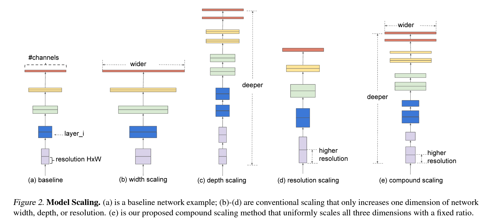
In this paper, we want to study and rethink the process of scaling up ConvNets. In particular, we investigate the central question: is there a principled method to scale up ConvNets that can achieve better accuracy and efficiency? Our empirical study shows that it is critical to balance all dimensions of network width/depth/resolution, and surprisingly such balance can be achieved by simply scaling each of them with constant ratio. Based on this observation, we propose a simple yet effective compound scaling method. Unlike conventional practice that arbitrary scales these factors, our method uniformly scales network width, depth, and resolution with a set of fixed scaling coefficients. For example, if we want to use 2N times more computational resources, then we can simply increase the network depth by αN , width by βN , and image size by γN , where α, β, γ are constant coefficients determined by a small grid search on the original small model. Figure 2 illustrates the difference between our scaling method and conventional methods.
Figure 2. Model Scaling. (a) is a baseline network example; (b)-(d) are conventional scaling that only increases one dimension of network width, depth, or resolution. (e) is our proposed compound scaling method that uniformly scales all three dimensions with a fixed ratio.
Intuitively, the compound scaling method makes sense because if the input image is bigger, then the network needs more layers to increase the receptive field and more channels to capture more fine-grained patterns on the bigger image. In fact, previous theoretical (Raghu et al., 2017; Lu et al., 2018) and empirical results (Zagoruyko & Komodakis, 2016) both show that there exists certain relationship between network width and depth, but to our best knowledge, we are the first to empirically quantify the relationship among all three dimensions of network width, depth, and resolution.
We demonstrate that our scaling method work well on existing MobileNets (Howard et al., 2017; Sandler et al., 2018) and ResNet (He et al., 2016). Notably, the effectiveness of model scaling heavily depends on the baseline network; to go even further, we use neural architecture search (Zoph & Le, 2017; Tan et al., 2019) to develop a new baseline network, and scale it up to obtain a family of models, called EfficientNets. Figure 1 summarizes the ImageNet performance, where our EfficientNets significantly outperform other ConvNets. In particular, our EfficientNet-B7 surpasses the best existing GPipe accuracy (Huang et al., 2018), but using 8.4x fewer parameters and running 6.1x faster on inference. Compared to the widely used ResNet-50 (He et al., 2016), our EfficientNet-B4 improves the top-1 accuracy from 76.3% to 83.0% (+6.7%) with similar FLOPS. Besides ImageNet, EfficientNets also transfer well and achieve state-of-the-art accuracy on 5 out of 8 widely used datasets, while reducing parameters by up to 21x than existing ConvNets.
2. Related Work
ConvNet Accuracy: Since AlexNet (Krizhevsky et al., 2012) won the 2012 ImageNet competition, ConvNets have become increasingly more accurate by going bigger: while the 2014 ImageNet winner GoogleNet (Szegedy et al., 2015) achieves 74.8% top-1 accuracy with about 6.8M parameters, the 2017 ImageNet winner SENet (Hu et al., 2018) achieves 82.7% top-1 accuracy with 145M parameters. Recently, GPipe (Huang et al., 2018) further pushes the state-of-the-art ImageNet top-1 validation accuracy to 84.3% using 557M parameters: it is so big that it can only be trained with a specialized pipeline parallelism library by partitioning the network and spreading each part to a different accelerator. While these models are mainly designed for ImageNet, recent studies have shown better ImageNet models also perform better across a variety of transfer learning datasets (Kornblith et al., 2019), and other computer vision tasks such as object detection (He et al., 2016; Tan et al., 2019). Although higher accuracy is critical for many applications, we have already hit the hardware memory limit, and thus further accuracy gain needs better efficiency.
ConvNet Efficiency: Deep ConvNets are often overparameterized. Model compression (Han et al., 2016; He et al., 2018; Yang et al., 2018) is a common way to reduce model size by trading accuracy for efficiency. As mobile phones become ubiquitous, it is also common to handcraft efficient mobile-size ConvNets, such as SqueezeNets (Iandola et al., 2016; Gholami et al., 2018), MobileNets (Howard et al., 2017; Sandler et al., 2018), and ShuffleNets(Zhang et al., 2018; Ma et al., 2018). Recently, neural architecture search becomes increasingly popular in designing efficient mobile-size ConvNets (Tan et al., 2019; Cai et al., 2019), and achieves even better efficiency than hand-crafted mobile ConvNets by extensively tuning the network width, depth, convolution kernel types and sizes. However, it is unclear how to apply these techniques for larger models that have much larger design space and much more expensive tuning cost. In this paper, we aim to study model efficiency for super large ConvNets that surpass state-of-the-art accuracy. To achieve this goal, we resort to model scaling.
Model Scaling: There are many ways to scale a ConvNet for different resource constraints: ResNet (He et al., 2016) can be scaled down (e.g., ResNet-18) or up (e.g., ResNet-200) by adjusting network depth (#layers), while WideResNet (Zagoruyko & Komodakis, 2016) and MobileNets (Howard et al., 2017) can be scaled by network width (#channels). It is also well-recognized that bigger input image size will help accuracy with the overhead of more FLOPS. Although prior studies (Raghu et al., 2017; Lin & Jegelka, 2018; Sharir & Shashua, 2018; Lu et al., 2018) have shown that network depth and width are both important for ConvNets’ expressive power, it still remains an open question of how to effectively scale a ConvNet to achieve better efficiency and accuracy. Our work systematically and empirically studies ConvNet scaling for all three dimensions of network width, depth, and resolutions.
Figure 2(a) illustrate a representative ConvNet, where the spatial dimension is gradually shrunk but the channel dimension is expanded over layers, for example, from initial input shape (cid:104)224, 224, 3(cid:105) to final output shape (cid:104)7, 7, 512(cid:105).
Unlike regular ConvNet designs that mostly focus on finding the best layer architecture Fi, model scaling tries to expand the network length (Li), width (Ci), and/or resolution (Hi, Wi) without changing Fi predefined in the baseline network. By fixing Fi, model scaling simplifies the design problem for new resource constraints, but it still remains a large design space to explore different Li, Ci, Hi, Wi for each layer. In order to further reduce the design space, we restrict that all layers must be scaled uniformly with constant ratio. Our target is to maximize the model accuracy for any given resource constraints, which can be formulated as an optimization problem:
where w, d, r are coefficients for scaling network width, depth, and resolution; ˆFi, ˆLi, ˆHi, ˆWi, ˆCi are predefined parameters in baseline network (see Table 1 as an example).
3. Compound Model Scaling
3.2. Scaling Dimensions
In this section, we will formulate the scaling problem, study different approaches, and propose our new scaling method.
3.1. Problem Formulation
A ConvNet Layer i can be defined as a function: Yi = Fi(Xi), where Fi is the operator, Yi is output tensor, Xi is input tensor, with tensor shape (cid:104)Hi, Wi, Ci(cid:105)1, where Hi and Wi are spatial dimension and Ci is the channel dimension. A ConvNet N can be represented by a list of composed layers: N = Fk (cid:12) … (cid:12) F2 (cid:12) F1(X1) = (cid:74) j=1…k Fj(X1). In practice, ConvNet layers are often partitioned into multiple stages and all layers in each stage share the same architecture: for example, ResNet (He et al., 2016) has five stages, and all layers in each stage has the same convolutional type except the first layer performs down-sampling. Therefore, we can define a ConvNet as:
where F Li i denotes layer Fi is repeated Li times in stage i, (cid:104)Hi, Wi, Ci(cid:105) denotes the shape of input tensor X of layer
1 For the sake of simplicity, we omit batch dimension.
The main difficulty of problem 2 is that the optimal d, w, r depend on each other and the values change under different resource constraints. Due to this difficulty, conventional methods mostly scale ConvNets in one of these dimensions:
Depth (ddd): Scaling network depth is the most common way used by many ConvNets (He et al., 2016; Huang et al., 2017; Szegedy et al., 2015; 2016). The intuition is that deeper ConvNet can capture richer and more complex features, and generalize well on new tasks. However, deeper networks are also more difficult to train due to the vanishing gradient problem (Zagoruyko & Komodakis, 2016). Although several techniques, such as skip connections (He et al., 2016) and batch normalization (Ioffe & Szegedy, 2015), alleviate the training problem, the accuracy gain of very deep network diminishes: for example, ResNet-1000 has similar accuracy as ResNet-101 even though it has much more layers. Figure 3 (middle) shows our empirical study on scaling a baseline model with different depth coefficient d, further suggesting the diminishing accuracy return for very deep ConvNets.
Width (www): Scaling network width is commonly used for small size models (Howard et al., 2017; Sandler et al., 2018; Tan et al., 2019) As discussed in (Zagoruyko & Komodakis, 2016), wider networks tend to be able to capture more fine-grained features and are easier to train. However, extremely wide but shallow networks tend to have difficulties in capturing higher level features. Our empirical results in Figure 3 (left) show that the accuracy quickly saturates when networks become much wider with larger w.
Figure 3. Scaling Up a Baseline Model with Different Network Width (w), Depth (d), and Resolution (r) Coefficients. Bigger networks with larger width, depth, or resolution tend to achieve higher accuracy, but the accuracy gain quickly saturate after reaching 80%, demonstrating the limitation of single dimension scaling. Baseline network is described in Table 1.
Resolution (rrr): With higher resolution input images, ConvNets can potentially capture more fine-grained patterns. Starting from 224x224 in early ConvNets, modern ConvNets tend to use 299x299 (Szegedy et al., 2016) or 331x331 (Zoph et al., 2018) for better accuracy. Recently, GPipe (Huang et al., 2018) achieves state-of-the-art ImageNet accuracy with 480x480 resolution. Higher resolutions, such as 600x600, are also widely used in object detection ConvNets (He et al., 2017; Lin et al., 2017). Figure 3 (right) shows the results of scaling network resolutions, where indeed higher resolutions improve accuracy, but the accuracy gain diminishes for very high resolutions (r = 1.0 denotes resolution 224x224 and r = 2.5 denotes resolution 560x560).
The above analyses lead us to the first observation:
- Observation 1: Scaling up any dimension of network width, depth, or resolution improves accuracy, but the accuracy gain diminishes for bigger models.
#3.3. Compound Scaling
We empirically observe that different scaling dimensions are not independent. Intuitively, for higher resolution images, we should increase network depth, such that the larger receptive fields can help capture similar features that include more pixels in bigger images. Correspondingly, we should also increase network width when resolution is higher, in order to capture more fine-grained patterns with more pixels in high resolution images. These intuitions suggest that we need to coordinate and balance different scaling dimensions rather than conventional single-dimension scaling.
2 In some literature, scaling number of channels is called “depth multiplier”, which means the same as our width coefficient w.
Figure 4. Scaling Network Width for Different Baseline Networks. Each dot in a line denotes a model with different width coefficient (w). All baseline networks are from Table 1. The first baseline network (d=1.0, r=1.0) has 18 convolutional layers with resolution 224x224, while the last baseline (d=2.0, r=1.3) has 36 layers with resolution 299x299.
To validate our intuitions, we compare width scaling under different network depths and resolutions, as shown in Figure 4. If we only scale network width w without changing depth (d=1.0) and resolution (r=1.0), the accuracy saturates quickly. With deeper (d=2.0) and higher resolution (r=2.0), width scaling achieves much better accuracy under the same FLOPS cost. These results lead us to the second observation:
- Observation 2: In order to pursue better accuracy and efficiency, it is critical to balance all dimensions of network width, depth, and resolution during ConvNet scaling.
In fact, a few prior work (Zoph et al., 2018; Real et al., 2019) have already tried to arbitrarily balance network width and depth, but they all require tedious manual tuning.
Table 1. EfficientNet-B0 baseline network – Each row describes a stage i with ˆLi layers, with input resolution (cid:104) ˆHi, ˆWi(cid:105) and output channels ˆCi. Notations are adopted from equation 2.
In this paper, we propose a new compound scaling method, which use a compound coefficient φ to uniformly scales network width, depth, and resolution in a principled way:
where α, β, γ are constants that can be determined by a small grid search. Intuitively, φ is a user-specified coefficient that controls how many more resources are available for model scaling, while α, β, γ specify how to assign these extra resources to network width, depth, and resolution respectively. Notably, the FLOPS of a regular convolution op is proportional to d, w2, r2, i.e., doubling network depth will double FLOPS, but doubling network width or resolution will increase FLOPS by four times. Since convolution ops usually dominate the computation cost in ConvNets, scaling a ConvNet with equation 3 will approximately increase total FLOPS by (cid:0)α · β2 · γ2(cid:1)φ . In this paper, we constraint α · β2 · γ2 ≈ 2 such that for any new φ, the total FLOPS will approximately3 increase by 2φ.
4. EfficientNet Architecture
Since model scaling does not change layer operators ˆFi in baseline network, having a good baseline network is also critical. We will evaluate our scaling method using existing ConvNets, but in order to better demonstrate the effectiveness of our scaling method, we have also developed a new mobile-size baseline, called EfficientNet.
Inspired by (Tan et al., 2019), we develop our baseline network by leveraging a multi-objective neural architecture search that optimizes both accuracy and FLOPS. Specifically, we use the same search space as (Tan et al., 2019), and use ACC(m)×[F LOP S(m)/T ]w as the optimization goal, where ACC(m) and F LOP S(m) denote the accuracy and FLOPS of model m, T is the target FLOPS and w=-0.07 is a hyperparameter for controlling the trade-off between accuracy and FLOPS. Unlike (Tan et al., 2019; Cai et al., 2019), here we optimize FLOPS rather than latency since we are not targeting any specific hardware device. Our search produces an efficient network, which we name EfficientNet-B0. Since we use the same search space as (Tan et al., 2019), the architecture is similar to Mnas-Net, except our EfficientNet-B0 is slightly bigger due to the larger FLOPS target (our FLOPS target is 400M). Table 1 shows the architecture of EfficientNet-B0. Its main building block is mobile inverted bottleneck MBConv (Sandler et al., 2018; Tan et al., 2019), to which we also add squeeze-and-excitation optimization (Hu et al., 2018).
3 FLOPS may differ from theoretical value due to rounding.
Starting from the baseline EfficientNet-B0, we apply our compound scaling method to scale it up with two steps:
• STEP 1: we first fix φ = 1, assuming twice more resources available, and do a small grid search of α, β, γ In particular, we find based on Equation 2 and 3. the best values for EfficientNet-B0 are α = 1.2, β = 1.1, γ = 1.15, under constraint of α · β2 · γ2 ≈ 2. • STEP 2: we then fix α, β, γ as constants and scale up baseline network with different φ using Equation 3, to obtain EfficientNet-B1 to B7 (Details in Table 2).
Notably, it is possible to achieve even better performance by searching for α, β, γ directly around a large model, but the search cost becomes prohibitively more expensive on larger models. Our method solves this issue by only doing search once on the small baseline network (step 1), and then use the same scaling coefficients for all other models (step 2).
5. Experiments
In this section, we will first evaluate our scaling method on existing ConvNets and the new proposed EfficientNets.
5.1. Scaling Up MobileNets and ResNets
As a proof of concept, we first apply our scaling method to the widely-used MobileNets (Howard et al., 2017; Sandler et al., 2018) and ResNet (He et al., 2016). Table 3 shows the ImageNet results of scaling them in different ways. Compared to other single-dimension scaling methods, our compound scaling method improves the accuracy on all these models, suggesting the effectiveness of our proposed scaling method for general existing ConvNets.
Table 2. EfficientNet Performance Results on ImageNet (Russakovsky et al., 2015). All EfficientNet models are scaled from our baseline EfficientNet-B0 using different compound coefficient φ in Equation 3. ConvNets with similar top-1/top-5 accuracy are grouped together for efficiency comparison. Our scaled EfficientNet models consistently reduce parameters and FLOPS by an order of magnitude (up to 8.4x parameter reduction and up to 16x FLOPS reduction) than existing ConvNets.
Figure 5. FLOPS vs. ImageNet Accuracy – Similar to Figure 1 except it compares FLOPS rather than model size.
5.2. ImageNet Results for EfficientNet
We train our EfficientNet models on ImageNet using similar settings as (Tan et al., 2019): RMSProp optimizer with decay 0.9 and momentum 0.9; batch norm momentum 0.99; weight decay 1e-5; initial learning rate 0.256 that decays by 0.97 every 2.4 epochs. We also use SiLU (Swish-1) activation (Ramachandran et al., 2018; Elfwing et al., 2018; Hendrycks & Gimpel, 2016), AutoAugment (Cubuk et al., 2019), and stochastic depth (Huang et al., 2016) with survival probability 0.8. As commonly known that bigger models need more regularization, we linearly increase dropout (Srivastava et al., 2014) ratio from 0.2 for EfficientNet-B0 to 0.5 for B7. We reserve 25K randomly picked images from the training set as a minival set, and perform early stopping on this minival; we then evaluate the earlystopped checkpoint on the original validation set to report the final validation accuracy.
Table 5. EfficientNet Performance Results on Transfer Learning Datasets. Our scaled EfficientNet models achieve new state-of-theart accuracy for 5 out of 8 datasets, with 9.6x fewer parameters on average.
Figure 6. Model Parameters vs. Transfer Learning Accuracy – All models are pretrained on ImageNet and finetuned on new datasets.
Table 2 shows the performance of all EfficientNet models that are scaled from the same baseline EfficientNet-B0. Our EfficientNet models generally use an order of magnitude fewer parameters and FLOPS than other ConvNets with similar accuracy. In particular, our EfficientNet-B7 achieves 84.3% top1 accuracy with 66M parameters and 37B FLOPS,
Figure 1 and Figure 5 illustrates the parameters-accuracy and FLOPS-accuracy curve for representative ConvNets, where our scaled EfficientNet models achieve better accuracy with much fewer parameters and FLOPS than other ConvNets. Notably, our EfficientNet models are not only small, but also computational cheaper. For example, our EfficientNet-B3 achieves higher accuracy than ResNeXt-101 (Xie et al., 2017) using 18x fewer FLOPS.
To validate the latency, we have also measured the inference latency for a few representative CovNets on a real CPU as shown in Table 4, where we report average latency over 20 runs. Our EfficientNet-B1 runs 5.7x faster than the widely used ResNet-152, while EfficientNet-B7 runs about 6.1x faster than GPipe (Huang et al., 2018), suggesting our EfficientNets are indeed fast on real hardware.
Table 6. Transfer Learning Datasets.
5.3. Transfer Learning Results for EfficientNet
We have also evaluated our EfficientNet on a list of commonly used transfer learning datasets, as shown in Table 6. We borrow the same 훈련 설정s from (Kornblith et al., 2019) and (Huang et al., 2018), which take ImageNet pretrained checkpoints and finetune on new datasets.
Table 5 shows the transfer learning performance: (1) Compared to public available models, such as NASNet-A (Zoph et al., 2018) and Inception-v4 (Szegedy et al., 2017), our EfficientNet models achieve better accuracy with 4.7x average (up to 21x) parameter reduction. (2) Compared to stateof-the-art models, including DAT (Ngiam et al., 2018) that dynamically synthesizes training data and GPipe (Huang et al., 2018) that is trained with specialized pipeline parallelism, our EfficientNet models still surpass their accuracy in 5 out of 8 datasets, but using 9.6x fewer parameters
Figure 6 compares the accuracy-parameters curve for a variety of models. In general, our EfficientNets consistently achieve better accuracy with an order of magnitude fewer parameters than existing models, including ResNet (He et al., 2016), DenseNet (Huang et al., 2017), Inception (Szegedy et al., 2017), and NASNet (Zoph et al., 2018).
6. Discussion
To disentangle the contribution of our proposed scaling method from the EfficientNet architecture, Figure 8 compares the ImageNet performance of different scaling meth-
Figure 8. Scaling Up EfficientNet-B0 with Different Methods.
Table 7. Scaled Models Used in Figure 7.
In order to further understand why our compound scaling method is better than others, Figure 7 compares the class activation map (Zhou et al., 2016) for a few representative models with different scaling methods. All these models are scaled from the same baseline, and their statistics are shown in Table 7. Images are randomly picked from ImageNet validation set. As shown in the figure, the model with compound scaling tends to focus on more relevant regions with more object details, while other models are either lack of object details or unable to capture all objects in the images.
7. Conclusion
In this paper, we systematically study ConvNet scaling and identify that carefully balancing network width, depth, and resolution is an important but missing piece, preventing us from better accuracy and efficiency. To address this issue, we propose a simple and highly effective compound scaling method, which enables us to easily scale up a baseline ConvNet to any target resource constraints in a more principled way, while maintaining model efficiency. Powered by this compound scaling method, we demonstrate that a mobilesize EfficientNet model can be scaled up very effectively, surpassing state-of-the-art accuracy with an order of magnitude fewer parameters and FLOPS, on both ImageNet and five commonly used transfer learning datasets.