Attention | Lightning Attention 2

• Related Project: Private
• Category: Paper Review
• Date: 2024-01-09

Lightning Attention-2: A Free Lunch for Handling Unlimited Sequence Lengths in Large Language Models

• url: https://arxiv.org/abs/2401.04658
• pdf: https://arxiv.org/pdf/2401.04658
• abstract: Linear attention is an efficient attention mechanism that has recently emerged as a promising alternative to conventional softmax attention. With its ability to process tokens in linear computational complexities, linear attention, in theory, can handle sequences of unlimited length without sacrificing speed, i.e., maintaining a constant training speed for various sequence lengths with a fixed memory consumption. However, due to the issue with cumulative summation (cumsum), current linear attention algorithms cannot demonstrate their theoretical advantage in a causal setting. In this paper, we present Lightning Attention-2, the first linear attention implementation that enables linear attention to realize its theoretical computational benefits. To achieve this, we leverage the thought of tiling, separately handling the intra-block and inter-block components in linear attention calculation. Specifically, we utilize the conventional attention computation mechanism for the intra-blocks and apply linear attention kernel tricks for the inter-blocks. A tiling technique is adopted through both forward and backward procedures to take full advantage of the GPU hardware. We implement our algorithm in Triton to make it IO-aware and hardware-friendly. Various experiments are conducted on different model sizes and sequence lengths. Lightning Attention-2 retains consistent training and inference speed regardless of input sequence length and is significantly faster than other attention mechanisms. The source code is available at this https URL.

Contents

• Lightning Attention-2: A Free Lunch for Handling Unlimited Sequence Lengths in Large Language Models
  • TL;DR
  • 1 Introduction
  • 2. Related Work
    • 2.1. Linear Attention
    • 2.2. IO-aware Attention
    • 2.3. Long Sequence Handling in LLM
  • 3. Method
    • 3.1. Preliminary
    • 3.2. Lightning Attention-2
      • 3.2.1. Forward Pass
        • Algorithm 1: Lightning Attention-2 Forward Pass
      • 3.2.2. Backward Pass
        • Algorithm 2: Lightning Attention-2 Backward Pass
  • 4. Experiments
    • 4.1. Attention Module Evaluation
    • 4.2. Lightning Attention-2 in Large Language Model
    • 4.3. Benchmarking Lightning Attention-2 in Large
  • 5. Conclusion

TL;DR

• Linear-attention기법을 활용한 LLM의 연산 복잡성 감소
• 속도 향상과 메모리 최적화를 위한 Lightning Attention-2 방법 제안
• 다양한 시퀀스 길이에서의 효율성 및 성능 검증

1 서론

대규모 언어모델(Large Language Models, LLM)은 다양한 전문 분야에서 확장된 대화나 대량의 토큰을 처리하는 등의 응용 가능성 때문에 많은 관심을 받고 있다. 이런 모델들은 입력 시퀀스 길이에 따라 계산 복잡도가 기하급수적으로 증가하는 문제가 있으며, 특히 이는 $O(n^2)$로 표현할 수 있습니다. 이런 문제를 해결하기 위해 linear attention 기법이 제안되었다. linear attention는 softmax 연산을 제거하고, 행렬 곱의 결합 법칙을 이용하여 계산 복잡도를 $O(n)$으로 감소시킨다. 이 연구에서는 Lightning Attention-2(Lightning Attention-2)를 도입하여 linear attention의 계산 복잡성을 극복하고자 합니다.

2 관련 연구

2.1 linear attention

선형 트랜스포머 구조는 기존의 Softmax 주의 메커니즘을 다양한 근사 방법으로 대체할 수 있습니다. 예를 들어, Katharopoulos 등(2020)은 1 + elu 활성 함수를 사용하고, Qin 등(2022)은 코사인 함수로 softmax의 특성을 근사할 수 있습니다. 이런 방법들은 이론적으로는 $O(nd^2)$의 복잡성을 가지나, 실제로는 linear attention가 인과적 상황에서 cumsum 연산이 필요하기 때문에 계산 효율이 크게 떨어진다.

2.2 IO-인식 주의

FlashAttention 시리즈는 GPU 플랫폼에서 표준 주의 연산자를 효율적으로 구현하기 위한 시스템 수준의 최적화를 집중적으로 다루고, 이 접근 방식은 메모리 읽기/쓰기 양을 최소화하기 위해 타일링 전략을 사용합니다.

2.3 긴 시퀀스 처리

긴 시퀀스를 처리하기 위한 일반적인 전략은 상대적 위치 인코딩 기술을 통합하는 것으로, 예를 들어 Roformer는 rotation 위치 임베딩 방식을 소개하고, ALiBi는 주의 메커니즘에서 멀리 떨어진 토큰의 영향을 완화하는 전략을 취합니다.

이런 방법들은 주로 파인튜닝이나 테스트 단계에서 시퀀스 길이를 확장할 수 있으며, 본 연구에서 제안하는 방법은 처음부터 긴 시퀀스로 모델을 훈련할 수 있게 됩니다.

3 방법

3.1 기초

우선 linear attention의 기본 형식을 회고하고, Lightning Attention-2를 소개합니다. NormAttention은 기존 트랜스포머 구조에서 비용이 많이 드는 softmax 및 스케일링 연산을 생략합니다.

\(Q, K, V \in \mathbb{R}^{n \times d}\)는 각각 질의, 키, 값 행렬이며, \(n\)은 시퀀스 길이, \(d\)는 특징 차원을 나타냅니다. 행렬 곱을 통해 위 식을 선형 변형으로 수학적으로 동등하게 변환할 수 있습니다.

이 선형 형식은 반복 예측에 효율적인 \(O(nd^2)\)의 복잡성을 제공하고, linear attention는 시퀀스 길이에 관계없이 일정한 \(O(d^2)\)의 계산 복잡도를 보장하여 무한히 긴 시퀀스에 대한 인퍼런스를 가능하게 합니다.

그러나 인과적 예측 작업에서는 cumsum 연산의 필요성 때문에 우측 곱의 효과가 저하되므로, Lightning Attention-1에서는 전통적인 왼쪽 행렬 곱을 사용하여 이 문제를 해결하고자 합니다.

3.2 Lightning Attention-2

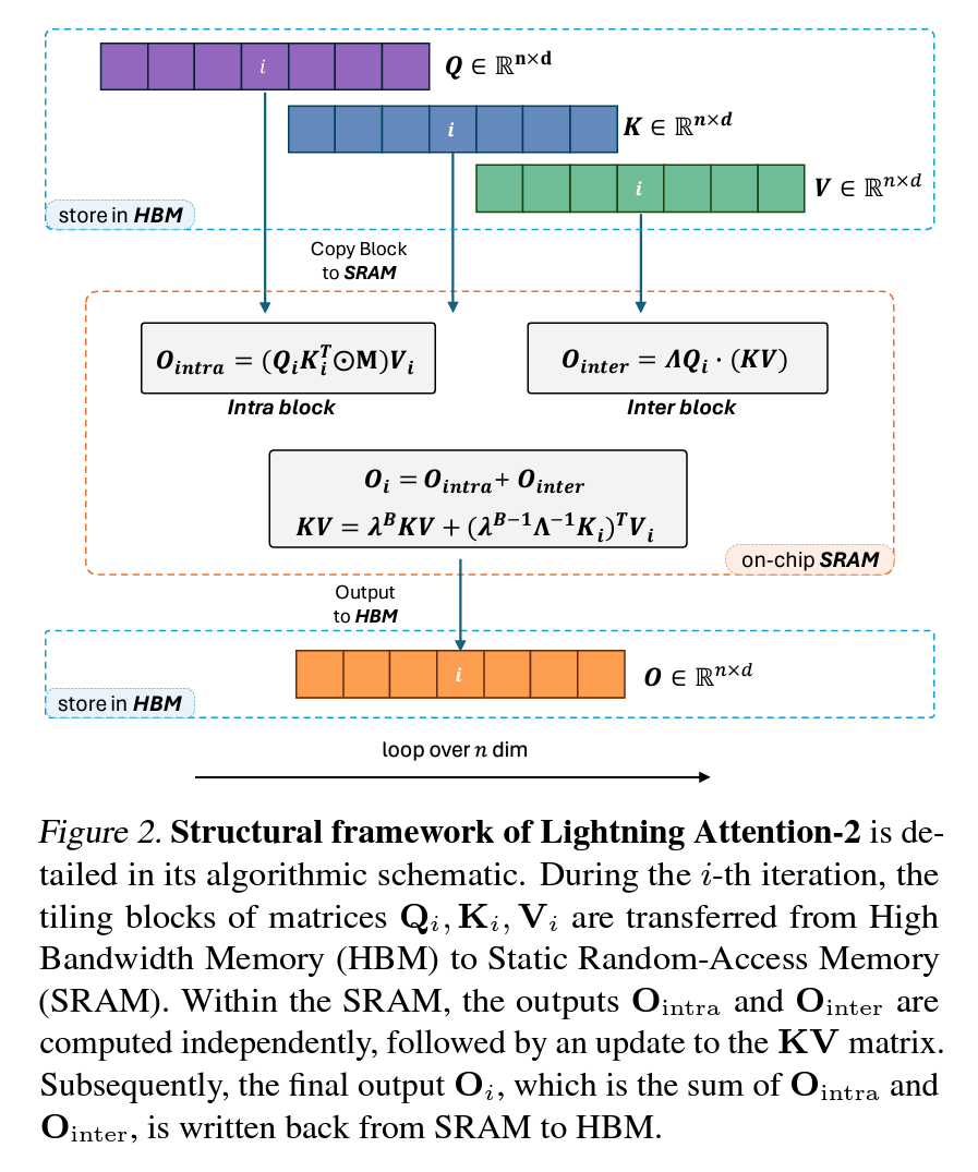
Lightning Attention-2는 전체 연산 과정에서 타일링 방법을 사용합니다. 각 반복에서 \(Q_i, K_i, V_i\) 행렬은 블록으로 나뉘어져 SRAM으로 전송되어 계산되며, 내부 블록에서는 왼쪽 곱을 사용하고, 외부 블록에서는 오른쪽 곱을 사용합니다.

이 접근 방식은 계산 및 메모리 효율을 최적화하여 전체 실행 속도를 향상시키고, 중간 활성화 \(KV\)는 SRAM 내에서 반복적으로 저장 및 누적되면서 내부 및 외부 블록의 출력은 SRAM 내에서 합산되기때문에 최종적으로 HBM으로 다시 쓰여지게 됩니다.

이 방법은 각 메모리 구성 요소의 독특한 이점을 활용하여 계산 워크플로를 최적화합니다.

알고리즘 1: Lightning Attention-2 정방향 패스

1. 입력과 초기 설정
   • $Q, K, V$는 크기 $n \times d$의 행렬이고, 감쇠율 $\lambda$는 양의 실수
   • 행렬 $X$를 $T = \frac{n}{B}$개의 블록 $X_1, X_2, \ldots, X_T$로 나누며, 각 블록의 크기는 $B \times d$
   • 마스크 $M$을 $B \times B$ 크기로 초기화하며, $M_{ij} = \lambda^{i-j}$ (단, $i \geq j$일 경우), 그렇지 않으면 0.
   • $\Lambda$를 대각 행렬로 초기화, $\Lambda = \text{diag}{\lambda, \lambda^2, \ldots, \lambda^B}$, 크기는 $B \times B$
   • $KV$를 $d \times d$ 크기의 0 행렬로 초기화
2. 반복 과정
   • $i = 1$부터 $T$까지 반복
     • $Q_i, K_i, V_i$ (크기 $B \times d$)를 HBM에서 온칩 SRAM으로 로드
     • 온칩에서 $O_{\text{intra}} = [(Q_i K_i^\top) \odot M] V_i$ 계산
     • 온칩에서 $O_{\text{inter}} = \Lambda Q_i (KV)$ 계산
     • 온칩에서 $KV$ 업데이트: $KV = \lambda^B KV + \lambda^B \Lambda^{-1} K_i)^\top V_i$.
     • $i$번째 블록의 결과 $O_i = O_{\text{intra}} + O_{\text{inter}}$를 HBM에 기록
3. 출력
   • $O$ 반환

Lightning Attention-2의 정방향 패스는 대략적으로 다음과 같은 과정을 거칩니다.

1. 입력 및 초기화: 입력 텐서 \(Q, K, V\)와 감쇠율 \(\lambda\), 그리고 블록 크기 \(B\)를 기반으로 하여 필요한 구조를 설정합니다.
2. 블록 나누기: 전체 텐서를 \(T = \frac{n}{B}\) 블록으로 나누어 각 블록이 \(B \times d\)의 크기를 갖도록 합니다. 이는 데이터를 관리 가능한 단위로 분할하여 계산을 효율적으로 만듭니다.
3. 마스크 및 감쇠 행렬 초기화: 마스크 \(M\)은 요소별 곱셈을 위한 필터로 사용되며, 감쇠 행렬 \(\Lambda\)는 각 블록 간의 상호작용을 조절합니다.
4. 온칩 계산
   • Ointra 계산: 내부 블록 출력은 \(Q\)와 \(K\)의 곱을 마스크 \(M\)과 요소별로 곱한 후 \(V\)와 곱합니다.
   • Ointer 계산: 외부 블록 출력은 감쇠 행렬 \(\Lambda\)를 사용하여 이전 블록의 결과 \(KV\)와 현재 블록의 \(Q\)를 결합합니다.
   • KV 업데이트: \(KV\)는 현재 블록의 \(K\)와 \(V\)의 곱에 기존 \(KV\) 값에 감쇠율 \(\lambda^B\)를 곱한 값을 더하여 업데이트합니다.
5. HBM 기록: 계산된 결과를 HBM(High Bandwidth Memory)에 기록하여 다음 단계의 계산이나 최종 출력에 사용할 수 있도록 합니다.

Lightning Attention-2의 forward pass 동안, \(t\)번째 출력은 다음과 같이 계산할 수 있습니다.

블록 형태로 방정식을 작성하면, 전체 시퀀스 길이 \(n\)과 블록 크기 \(B\)를 고려하여 \(X\)는 \(\{X_1, X_2, ..., X_T\}\)로 나뉘어지며, 각 블록은 \(B \times d\) 크기를 가집니다.

3.2.2. 역방향 패스

알고리즘 2: Lightning Attention-2 역방향 패스

1. 입력과 초기 설정
   • $Q, K, V, dO$는 크기 $n \times d$의 입력 텐서이고, 감쇠율 $\lambda$는 양의 실수, 블록 크기는 $B$입니다.
   • $X \in {Q, K, V}$를 $T = \frac{n}{B}$ 블록으로 나누고, 각 블록의 크기는 $B \times d$입니다.
   • $dX \in {dQ, dK, dV, dO}$도 $T = \frac{n}{B}$ 블록으로 나눕니다.
   • 마스크 $M$을 $B \times B$ 크기로 초기화하며, $M_{ij} = \lambda^{i-j}$ (단, $i \geq j$일 경우), 그렇지 않으면 0입니다.
   • $\Lambda$를 대각 행렬로 초기화, $\Lambda = \text{diag}{\lambda, \lambda^2, \ldots, \lambda^B}$, 크기는 $B \times B$입니다.
   • $KV$와 $dKV$를 $d \times d$ 크기의 0 행렬로 초기화합니다.
2. 정방향 패스
   • $i = 1$부터 $T$까지 반복하면서, $K_i, V_i, O_i, dO_i$를 HBM에서 온칩 SRAM으로 로드합니다.
   • 온칩에서 $dQ_{\text{intra}} = [(dO_i V_i^\top) \odot M] K_i$와 $dQ_{\text{inter}} = \Lambda dO_i (KV)^\top$를 계산합니다.
   • $KV$를 $\lambda^B KV + \lambda^B \Lambda^{-1} K_i)^\top V_i$로 업데이트합니다.
   • $dQ_i = dQ_{\text{intra}} + dQ_{\text{inter}}$를 HBM에 기록합니다.
3. 역방향 패스
   • $i = T$부터 1까지 반복하면서, $Q_i, K_i, V_i, O_i, dO_i$를 HBM에서 온칩 SRAM으로 로드합니다.
   • 온칩에서 $dK_{\text{intra}} = [(dO_i V_i^\top) \odot M]^\top Q_i$, $dK_{\text{inter}} = \lambda^B \Lambda^{-1} V_i) (dKV)^\top$, $dV_{\text{intra}} = [(Q_i K_i^\top) \odot M]^\top dO_i$, $dV_{\text{inter}} = \lambda^B \Lambda^{-1} K_i) dKV$를 계산합니다.
   • $KV$를 $\lambda^B dKV + $$Lambda Q_i)^\top dO_i$로 업데이트합니다.
   • $dK_i = dK_{\text{intra}} + dK_{\text{inter}}$, $dV_i = dV_{\text{intra}} + dV_{\text{inter}}$를 HBM에 기록합니다.
4. 출력
   • $dQ, dK, dV$를 반환하여 질의, 키, 값에 대한 그래디언트 텐서를 제공합니다.

역방향 패스의 논리적 과정을 설명하기 위해, 주어진 \(do_t\)에 대해 다음과 같은 수식을 고려합니다.

\(dkv_t\)를 재귀적 형태로 쓰면, 다음과 같이 표현됩니다.

전체 시퀀스 길이 \(n\)과 블록 크기 \(B\)를 고려할 때, \(X\)는 크기 \(B \times d\)를 가진 블록 \(\{X_1, X_2, ..., X_T\}\)로 나누어집니다. 이를 바탕으로 블록 스타일의 방정식을 다음과 같이 작성할 수 있습니다.

그리고 \((t+1)\)번째 블록, 즉 \(tB+r\), \(0 \leq r < B\)에 대해,

행렬 형식으로 표현하면,

이와 같이 역방향 패스의 각 단계는 블록 간의 그래디언트 전파와 누적을 통해 계산을 효율적으로 수행하며, Lightning Attention-2의 전체적인 메모리 및 계산 최적화를 가능하게 합니다.

Linear Attention의 개선 참고자료: Zoology (Blogpost 2): Simple, Input-Dependent, and Sub-Quadratic Sequence Mixers

1 Introduction

(LLM) (Brown et al., 2020; Touvron et al., 2023a;b; Peng et al., 2023; Qin et al., 2023b) and multi-modal models (Li et al., 2022; 2023a; Liu et al., 2023; Radford et al., 2021; Li et al., 2023b; Lu et al., 2022; Mao et al., 2023; Shen et al., 2023; Zhou et al., 2023; Sun et al., 2023a; Hao et al., 2024). However, its computational complexity grows quadratically with the length of the input sequence, making it challenging to model extremely long sequences.

Unlimited sequence length stands out as a noteworthy aspect within the realm of LLM, attracting considerable attention from researchers who seek intelligent solutions. The potential applications of LLM with unlimited sequence length are diverse, encompassing extended conversations in various professional domains and handling a vast number of tokens in multimodal modeling tasks.

In response to the quadratic complexity challenge, a promising resolution emerges in the form of linear attention. This method involves the elimination of the softmax operation and capitalizes on the associativity property of matrix products. Consequently, it significantly accelerates both training and inference procedures. To elaborate, linear attention reduces the computational complexity from O(n2) to O(n) by leveraging the kernel trick (Katharopoulos et al., 2020b; Choromanski et al., 2020; Peng et al., 2021; Qin et al., 2022b) to compute the attention matrices, where n represents the sequence length. This avenue holds substantial promise for augmenting the efficiency of transformer-style models across a broad spectrum of applications.

It is important to note that the notable reduction in complexity from O(n2) to O(n) in linear attention is only theoretical and may not directly translate to a proportional improvement in computational efficiency on hardware in practice. The realization of practical wall-clock speedup faces challenges, primarily stemming from two issues: 1) the dominance of memory access (I/O) on the GPU could impact the overall computation speed of attention. 2) the cumulative summation (cumsum) needed by the linear attention kernel trick prevents it from reaching its theoretical training speed in the causal setting.

The first issue has been successfully addressed by Lightning Attention-1 (Qin et al., 2023b). In this paper, we introduce Lightning Attention-2 to solve the second issue. The key idea is to leverage the concept of “divide and conquer” by separately handling the intra block and inter block components in linear attention calculation. Specifically, for the intra blocks, we maintain the use of conventional attention computation mechanism to compute the product of QKV, while for the inter blocks, we employ the linear attention kernel trick (Katharopoulos et al., 2020b). Tiling techniques are implemented in both forward and backward procedures to fully leverage GPU hardware capabilities. As a result, the Lightning Attention-2 can train LLMs with unlimited sequence length without extra cost1, as its computational speed remains constant with increasing sequence length under fixed memory consumption.

Figure 1. Speed Showdown: FlashAttention vs. Lightning Attention in Expanding Sequence Lengths and Model Sizes. The diagram above provides a comparative illustration of training speed, Token per GPU per Second (TGS) for LLaMA with FlashAttention-2, TransNormerLLM with Lightning Attention-1 and TransNormerLLM with Lightning Attention-2, implemented across three model sizes: 400M, 1B, and 3B from left to right. It is strikingly evident that Lightning Attention-2 manifests a consistent training speed irrespective of the increasing sequence length. Conversely, the other methods significantly decline training speed as the sequence length expands.

We performed a comprehensive evaluation of Lightning Attention-2 across a diverse range of sequence lengths to assess its accuracy and compare its computational speed and memory utilization with FlashAttention-2 (Dao, 2023) and Lightning Attention-1. The findings indicate that Lightning Attention-2 exhibits a notable advantage in computational speed, attributed to its innovative intra-inter separation strategy. Additionally, Lightning Attention-2 demonstrates a reduced memory footprint compared to its counterparts without compromising performance.

2. Related Work

2.1. Linear Attention

Linear Transformer architectures discard the Softmax Attention mechanism, replacing it with distinct approximations (Katharopoulos et al., 2020a; Choromanski et al., 2020; Peng et al., 2021; Qin et al., 2022b;a). The key idea is to leverage the “kernel trick” to accelerate the attention matrix computation, i.e., compute the product of keys and values first to circumvent the n × n matrix multiplication. Multiple methods have been proposed to replace the softmax operation. For instance, Katharopoulos et al. (2020a) employ the 1 + elu activation function, Qin et al. (2022b) utilize the cosine function to approximate softmax properties, and Ke et al. (2021); Zheng et al. (2022; 2023) leverage sampling strategies to directly mimic softmax operation. Despite having a theoretical complexity of O(nd2), the practical computational efficiency of linear attention diminishes notably in causal attention scenarios, primarily due to the necessity for cumsum operations (Hua et al., 2022).

1 However, the sequence length may still be limited by hardware constraints, such as the GPU memory.

2.2. IO-aware Attention

The FlashAttention series (Dao et al., 2022; Dao, 2023) focuses on system-level optimizations for the efficient implementation of the standard attention operator on GPU platforms. Extensive validation has demonstrated its effectiveness. The approach employs tiling strategies to minimize the volume of memory reads/writes between the GPU’s high bandwidth memory (HBM) and on-chip SRAM.

To address the issue of slow computation for Linear Attention in the causal setting, Lightning Attention 1 (Qin et al., 2023b) employs the approach of FlashAttention-1/2, which involves segmenting the inputs Q, K, V into blocks, transferring them from slow HBM to fast SRAM, and then computing the attention output with respect to these blocks. Subsequently, the final results are accumulated. Although this method is much more efficient than the PyTorch implementation, it does not take advantage of the computational characteristics inherent to Linear Attention, and the theoretical complexity remains O(n2d).

2.3. Long Sequence Handling in LLM

A widely adopted strategy to tackle challenges related to length extrapolation involves the integration of Relative Positional Encoding (RPE) techniques (Su et al., 2021; Qin et al., 2023c), strategically directing attention towards neighboring tokens. ALiBi (Press et al., 2022) utilizes linear decay biases in attention mechanisms to mitigate the impact of distant tokens. Roformer (Su et al., 2021) introduces a novel Rotary Position Embedding (RoPE) method, widely embraced in the community, effectively leveraging positional information for transformer-based language model learning. Kerple (Chi et al., 2022) explores shift-invariant conditionally positive definite kernels within RPEs, introducing a suite of kernels aimed at enhancing length extrapolation properties, with ALiBi recognized as one of its instances. Furthermore, Sandwich (Chi et al., 2023) postulates a hypothesis elucidating the mechanism behind ALiBi, empirically validating it by incorporating the hypothesis into sinusoidal positional embeddings. (Qin et al., 2024) explored the sufficient conditions for additive relative position encoding to have extrapolation capabilities.

Instead of investigating the length extrapolation capability of transformers, some works also attempt to directly increase the context window sizes. Chen et al. (2023) introduces Position Interpolation (PI), extending context window sizes of RoPE-based pretrained Large Language Models (LLMs) such as LLaMA models to up to 32768 with minimal fine-tuning (within 1000 steps). StreamingLLM (Xiao et al., 2023) proposes leveraging the attention sink phenomenon, maintaining the Key and Value information of initial tokens to substantially recover the performance of window attention. As the sequence grows longer, the performance degrades. These methods can only extend sequence length in fine-tuning or testing phases, while our method allows training models in long sequence lengths from scratch with no additional cost.

3. Method

3.1. Preliminary

We first recall the formulation of linear attention and then introduce our proposed Lightning Attention-2. In the case of NormAttention within TransNormer (Qin et al., 2022a), attention computation deviates from the conventional Transformer structure (Vaswani et al., 2017) by eschewing the costly softmax and scaling operations. The NormAttention mechanism can be expressed as follows:

where $Q$, $K$, and $V \in \mathbb{R}^{n \times d}$ are the query, key, and value matrices, respectively, with $n$ denoting sequence length and $d$ representing feature dimension. To leverage the computational efficiency inherent in right matrix multiplication, the above equation can be seamlessly and mathematically equivalently transformed into its linear variant, as dictated by the properties of matrix multiplication:

This linear formulation facilitates recurrent prediction with a commendable complexity of $O(nd^2)$, rendering it efficient during training relative to sequence length. Furthermore, employing linear attention ensures a constant computation complexity of $O(d^2)$ irrespective of sequence length, thereby enabling inference over unlimited long sequences. This achievement is realized by updating $K^\top V$ recurrently without the need for repeated computation of the entire attention matrix.

In contrast, the standard softmax attention entails a computational complexity of $O(md^2)$ during the inference process, where $m$ denotes the token index. Nevertheless, when dealing with causal prediction tasks, the effectiveness of the right product is compromised, leading to the requirement for the computation of cumsum (Hua et al., 2022). This impediment hinders the potential for highly efficient parallel computation. Consequently, we persist with the conventional left matrix multiplication in Lightning Attention-1. This serves as the promotion behind the introduction of Lightning Attention-2, specifically crafted to address the challenges associated with the right product in such contexts.

3.2. Lightning Attention-2

Lightning Attention-2 employs a tiling methodology throughout its whole computation process. Given the huge variance in memory bandwidth between HBM and SRAM within GPU, Lightning Attention-2 applies a distinct strategy for leveraging them. In each iteration $i$, matrices $Q_i$, $K_i$, $V_i$ undergo segmentation into blocks, subsequently transferred to SRAM for computation. The intra- and inter-block operations are segregated, with intra-blocks employing the left product and inter-blocks utilizing the right product. This approach optimally exploits the computational and memory efficiencies associated with the right product, enhancing overall execution speed.

The intermediate activation $KV$ is iteratively saved and accumulated within SRAM. Subsequently, the outputs of intra-blocks and inter-blocks are summed within SRAM, and the results are written back to HBM. This method aims to capitalize on the distinct advantages of each memory component, optimizing the computational workflow.

The structural framework of Lightning Attention-2 is well illustrated in Fig. 2. The intricate details of the Lightning Attention-2 implementation are explicated through Algorithm 1 (forward pass) and Algorithm 2 (backward pass). These algorithms serve to encapsulate the nuanced computational procedures integral to Lightning Attention-2. Additionally, we provide a comprehensive derivation to facilitate a more profound comprehension of Lightning Attention-2. The derivations are systematically presented for both the forward pass and the backward pass, contributing to a thorough understanding of the underlying mechanisms.

3.2.1. Forward Pass

Algorithm 1: Lightning Attention-2 Forward Pass

Input: Q, K, V ∈ Rn×d, decay rate λ ∈ R+, block sizes B.
Divide X into T = n/B blocks X1, X2, ..., XT of size B × d each, where X ∈ {Q, K, V, O}.
Initialize mask M ∈ RB×B, where Mij = λi−j, if i ≥ j, else 0.
Initialize Λ = diag{λ, λ2, ..., λB} ∈ RB×B.
Initialize KV = 0 ∈ Rd×d.
for 1 ≤ i ≤ T do
    Load Qi, Ki, Vi ∈ RB×d from HBM to on-chip SRAM.
    On chip, compute Ointra = [(QiKi⊤) ⊙ M]Vi.
    On chip, compute Ointer = ΛQi(KV).
    On chip, compute KV = λBKV + (λBΛ−1Ki)⊤Vi.
    Write Oi = Ointra + Ointer to HBM as the i-th block of O.
end for
return O.

We ignore the $\text{Norm}(\cdot)$ operator in eq. (2) to simplify the derivations. During forward pass of Lightning Attention-2, the $t$-th output can be formulated as

In a recursive form, the above equation can be rewritten as

where

To perform tiling, let us write the equations in block form. Given the total sequence length $n$ and block size $B$, $X$ is divided into $T = \frac{n}{B}$ blocks ${X_1, X_2, …, X_T}$ of size $B \times d$ each, where $X \in {Q, K, V, O}$.

We first define

Given $KV_t$, the output of $(t+1)$-th block, i.e., $tB+r$, with $1 \leq r \leq B$ is

Rewritten in matrix form, we have

where

And the $KV$ at $(t+1)$-th block can be written as

The complete expression of the forward pass of Lightning Attention-2 can be found in Algorithm 1.

3.2.2. Backward Pass

Algorithm 2: Lightning Attention-2 Backward Pass

Input:

* Q, K, V, dO ∈ Rn×d: Input tensors (queries, keys, values, output gradients)
* decay_rate λ ∈ R+: Decay rate hyperparameter
* block_size B: Block size for memory chunking

Divide Inputs:

* Divide X ∈ {Q, K, V} into T = n/B blocks: X₁,...,XT of size B×d each.
* Divide dX ∈ {dQ, dK, dV, dO} into T = n/B blocks: dX₁,...,dX_T of size B×d each.

Initialization:

* M ∈ RB×B: Mask tensor, Mij = λ^(i-j) if i ≥ j, else 0.
* Λ = diag{λ, λ², ..., λ^B} ∈ RB×B: Diagonal matrix of decay rates.
* KV = 0, dKV = 0 ∈ Rd×d: Accumulators for key-value gradients and their updates.

Forward Pass (Loop 1):

1. For i = 1 to T:
    * Load Ki, Vi, Oi, dOi ∈ RB×d from HBM to on-chip SRAM.
    * On-chip computation:
        * dQ_intra = [(dOi * V⊤_i) ⊙ M] * Ki (element-wise multiplication with mask)
        * dQ_inter = Λ * dOi * (KV)⊤
    * On-chip update: KV = λ^B * KV + (λ^B * Λ⁻¹ * Ki)⊤ * Vi
    * Write dQi = dQ_intra + dQ_inter to HBM as the i-th block of dQ.

Backward Pass (Loop 2):

2. For i = T down to 1:
    * Load Qi, Ki, Vi, Oi, dOi ∈ RB×d from HBM to on-chip SRAM.
    * On-chip computation:
        * dK_intra = [(dOi * V⊤_i) ⊙ M]⊤ * Qi
        * dK_inter = (λ^B * Λ⁻¹ * Vi) * (dKV)⊤
        * dV_intra = [(Qi * K⊤_i) ⊙ M]⊤ * dOi
        * dV_inter = (λ^B * Λ⁻¹ * Ki) * dKV
    * On-chip update: KV = λ^B * dKV + (Λ * Qi)⊤ * dOi
    * Write dKi = dK_intra + dK_inter, dVi = dV_intra + dV_inter to HBM as the i-th block of dK, dV.

Output:

* Return dQ, dK, dV: Gradient tensors for queries, keys, and values.

For backward pass, let us consider the reverse process. First given $do_t$, we have

By writing $dkv_t$ in a recursive form, we get

To facilitate the understanding of tiling, let us consider the above equations in block style. Given the total sequence length $n$ and block size $B$, $X$ is divided into $T = \frac{n}{B}$ blocks ${X_1, X_2, …, X_T}$ of size $B \times d$ each, where $X \in {Q, K, V, O, dO}$.

We first define

Then for the $(t+1)$-th block, i.e., $tB+r$, $0 \leq r < B$, we have

In matrix form, we have

Since the recursion of $dK_t$ steps from $t+1$ to $t$, given $KV_{t+1}$, $dK_t$ for the $t$-th block, i.e., at positions $(t-1)B+r$, $0 < r \leq B$ is

In matrix form, we get

Considering $dV_t$ for the $t$-th block, i.e., at positions $(t-1)B+r$, $0 < r \leq B$, we have

In matrix form, we get

Finally, the recursive relation for $dKV_t$ is

\(\begin{aligned} dKV_t = \lambda_{s>t} B \lambda_{s-tB} q^\top s_{dos} \\ &= \lambda_B s > (t+1) B \lambda_{s-(t+1)B} q^\top s_{dos} + (t+1) B \lambda_{s=t+1} B \lambda_{s-tB} q^\top s_{dos} \\ &= \lambda_B dKV_{t+1} +\)Lambda^Q_t)^\top dO_t. (20) \end{aligned} $$

Algorithm 2 describes the backward pass of Lightning Attention-2 in more detail.

Discussion

A recent method, GLA (Yang et al., 2023), models sequences using linear attention with data-dependent decay. Its chunk-wise Block-Parallel Algorithm employs tiling and IO-aware concepts. However, unlike Lightning Attention-2, it uses parallel computations for each block, which leads to higher memory usage. Retnet (Sun et al., 2023b) is very similar in structure to TransNormer LLM (Qin et al., 2023b) and uses the chunk-wise retention algorithm. This algorithm is comparable to the forward pass of Lightning Attention-2 but does not consider IO-aware or the backward pass.

4. Experiments

To comprehensively assess Lightning Attention-2’s performance, speed, and memory utilization, we conducted extensive experiments on the TransNormerLLM model, with Lightning Attention-2 integrated. Our implementation utilizes the Metaseq framework (Zhang et al., 2022), a PyTorch-based sequence modeling framework (Paszke et al., 2019). All experiments are executed on the GPU cluster featuring 128 A100 80G GPUs. The deployment of Lightning Attention-2 is implemented in Triton (Tillet et al., 2019).

4.1. Attention Module Evaluation

We conducted a comparison of speed and memory usage among attention modules Lightning Attention-1, Lightning Attention-2, and FlashAttention-2, all under a single A100 80G GPU. As depicted in Figure 3, the analysis focuses on the runtime, measured in milliseconds, for the separated forward and backward propagation. The baseline runtime demonstrates a quadratic growth relative to the sequence length. In contrast, Lightning Attention-2 exhibits a markedly superior performance with linear growth. Notably, as the sequence length increases, this disparity in runtime becomes increasingly apparent. In addition to speed enhancements, our method also maintains a significant advantage in memory usage with the increase in sequence length.

Table 2. Language Modeling Comparison between TransNormer-LLM with Lightning Attention-1 and Lightning Attention-2.

4.2. Lightning Attention-2 in Large Language Model

Performance Evaluation In Table 2, we evaluated the performance of the TransNormerLLM-0.4B model under 2K contexts, comparing two variants: one equipped with Lightning Attention-1 and the other with Lightning Attention-2. These experiments were carried out using 8×A100 80G GPUs. After 100,000 iterations, using the sampled corpus from our corpus with 300B tokens and initial seed, we observed a marginal performance difference. Specifically, the variant with Lightning Attention-2 demonstrated a performance decrement of 0.001 compared to its counterpart with Lightning Attention-1.

Furthermore, our analysis extended to benchmarking the toptier efficient large language models, including LLaMA-FA2 (Touvron et al., 2023a; Dao, 2023), TNL-LA2, HGRN (Qin et al., 2023d), and TNN (Qin et al., 2023a). This benchmarking focused on training loss using a 30B subset of our uniquely assembled corpus, scaling from 1 to 3 billion parameters. As depicted in Figure 4, the TNL-LA2 model achieved marginally lower loss compared to the other models under review in both 1B and 3B parameters.

Figure 3. Comparative Analysis of Speed and Memory Usage: FlashAttention vs. Lightning Attention. Upper Section: Runtime in milliseconds for the forward and backward pass across varying sequence lengths. Lower Section: Memory utilization during the forward and backward pass at different sequence lengths.

Table 1. Efficiency Comparison of LLaMA with FlashAttention2, TransNormerLLM with Lightning Attention-1, and TransNormerLLM with Lightning Attention-2. The statistical analysis was performed using 2×A100 80G GPUs. The table reports Tokens per GPU per Second (TGS) across three different model sizes, within context ranges spanning from 1K to 92K. OOM stands for out of GPU memory.

Efficiency Evaluation In Table 1, we present a comparative analysis of training speeds under the same corpora and hardware setups. This comparison encompasses three variants: TransNormerLLM with Lightning Attention-2 (TNL-LA2), TransNormerLLM with Lightning Attention-1 (TNL-LA1), and LLaMA with FlashAttention2 (LLaMA-FA2). Our findings show that during both the forward and backward passes, the TGS (tokens per GPU per second) for TNL-LA2 remains consistently high, while the other two models exhibit a rapid decline when the sequence length is scaled from 1K to 92K. This pattern suggests that Lightning Attention-2 offers a significant advancement in managing unlimited sequence lengths in LLM.

4.3. Benchmarking Lightning Attention-2 in Large

Language Model

To evaluate the performance of the Lightning Attention-2, we conducted an analysis of the TransNormerLLM-15B (Qin et al., 2023b), a model comprising 15 billion parameters. The TransNormerLLM-15B is characterized by its 42 layers, 40 attention heads, and an overall embedding dimension of 5120. The model will be trained on a corpus of more than 1.3 trillion tokens with a sequence length of 6,144. Notably, the model achieved a processing speed of 1,620 tokens per GPU per second. Given that the comprehensive pre-training phase is scheduled to span three months, we hereby present the most recent results from the latest checkpoint for inclusion in Table 3.

Figure 4. Performance Comparison of HGRN, TNN, LLaMA with FlashAttention2 and TransNormerLLM with Lightning Attention-2. For the 1B model, we used 16×A800 80G GPUs with a batch size of 12 per GPU; for the 3B model, we scaled up to 32×A800 80G GPUs and a batch size of 30 per GPU. The training context length was set to 2K.

Table 3. Performance Comparison on Commonsense Reasoning and Aggregated Benchmarks. TNL-LA2: TransNormerLLM with Lightning Attention-2. PS: parameter size (billion). T: tokens (billion). HS: HellaSwag. WG: WinoGrande.

This evaluation is conducted using the lm-evaluation-harness framework (Gao et al., 2023). Our benchmark focuses on two key areas: Commonsense Reasoning (CSR) and Multiple Choice Questions (MCQ). For comparative analysis, we also evaluated the Pythia-12B (Biderman et al., 2023) model under the same benchmarks.

Commonsense Reasoning We report BoolQ (Clark et al., 2019), PIQA (Bisk et al., 2019), SIQA (Sap et al., 2019), HellaSwag (Zellers et al., 2019), WinoGrande (Sakaguchi et al., 2019), ARC easy and challenge (Clark et al., 2018), OpenBookQA (Mihaylov et al., 2018) and their average. In all CSR tasks, the performance of TransNormerLLM-15B surpassed Pythia-12B by about 2%. Furthermore, TransNormerLLM-15B-100B showed an approximate 3.5% improvement over its 50 billion-token stage, especially in the HellaSwag task, with over a 5% performance increase.

Aggregated Benchmarks We report the overall results for MMLU (Hendrycks et al., 2021) and C-Eval (Huang et al., 2023) with both 0-shot and 5-shot settings. In the C-Eval tasks, TransNormerLLM-15B is about 2% higher than Pythia-12B. In the 0-shot and 5-shot tests in both Chinese (C-Eval) and English (MMLU), TransNormerLLM-15B’s performance also exceeded the 25% baseline (the probability of random selection in a 4 choice scenario). We also noticed fluctuations in the 5-shot MCQ tasks, with an average MCQ score of around 26.5%.

5. Conclusion

In this paper, we introduced Lightning Attention-2, a pioneering implementation of linear attention that effectively harnesses its theoretical computational advantages, particularly in the causal setting. Our approach, which adopts the concepts of “divide and conquer” and tiling techniques, successfully addresses the limitations of current linear attention algorithms, especially the challenges associated with cumulative summation. By separating the computation into intrablock and inter-block components, we effectively leverage GPU hardware to its fullest potential, ensuring efficiency. Our extensive experiments across various model sizes and sequence lengths demonstrate that Lightning Attention-2 not only maintains consistent training speeds regardless of input sequence length but also outperforms existing state-of-the-art attention mechanisms in terms of speed and accuracy. This breakthrough has profound implications for the future of large language models, particularly those requiring the processing of long sequences. Looking ahead, we intend to introduce sequence parallelism in conjunction with Lightning Attention-2, which aims to facilitate the training of extralong sequences, effectively overcoming existing hardware constraints.