00:00:00

Iterative Data Smoothing**

https://dsdanielpark.github.io https://github.com/dsdanielpark

Iterative Data Smoothing**

MinWoo(Daniel) Park | Tech Blog

Created: 2024-01-30 22:36:30 +0000

Last modified: 2024-09-05 20:56:50 +0900

Iterative Data Smoothing**

Related Project: Private
Category: Paper Review
Date: 2024-01-31

Iterative Data Smoothing: Mitigating Reward Overfitting and Overoptimization in RLHF

url: https://arxiv.org/abs/2401.16335
pdf: https://arxiv.org/pdf/2401.16335
abstract: Reinforcement Learning from Human Feedback (RLHF) is a pivotal technique that aligns language models closely with human-centric values. The initial phase of RLHF involves learning human values using a reward model from ranking data. It is observed that the performance of the reward model degrades after one epoch of training, and optimizing too much against the learned reward model eventually hinders the true objective. This paper delves into these issues, leveraging the theoretical insights to design improved reward learning algorithm termed ‘Iterative Data Smoothing’ (IDS). The core idea is that during each training epoch, we not only update the model with the data, but also update the date using the model, replacing hard labels with soft labels. Our empirical findings highlight the superior performance of this approach over the traditional methods.

Contents

Iterative Data Smoothing: Mitigating Reward Overfitting and Overoptimization in RLHF

TL;DR

보상 학습과 정책 학습의 두 단계에서 발생하는 과적합 및 과최적화 문제 탐구
다중 팔 슬롯머신(Multi-Armed Bandits) 문제를 사용하여 이론적 해석 제공
효과적인 해결책으로 반복 데이터 평활화(IDS) 알고리즘 제안 및 검증

1. 서론

1.1 연구의 배경과 필요성

언어 모델의 파인튜닝 과정에서 휴먼의 평가를 통해 보상을 학습하는 방법인 Reinforcement Learning with Human Feedback (RLHF)은 자연어 처리 분야뿐만 아니라 다양한 인공지능 응용 분야에서 중요한 역할을 합니다. 그러나 RLHF의 전형적인 학습 과정에서는 데이터셋의 불균형으로 인해 발생하는 과적합 및 과최적화 문제가 종종 보고되어 왔습니다.

1.2 문제 정의

과적합은 모델이 training dataset에 지나치게 최적화되어 새로운 데이터에 대한 일반화 성능이 떨어지는 현상입니다. 과최적화는 보상 모델이 예측하는 보상을 극대화하려 할 때, 실제 보상과의 괴리가 커져서 최종적인 정책 모델의 성능이 저하되는 문제입니다.

2. 방법

2.1 RLHF의 일반적인 접근 방식

RLHF 프로세스는 크게 두 단계로 나뉩니다. 보상 학습과 정책 학습. 보상 학습 단계에서는 프롬프트와 여러 응답 사이의 선호도를 비교하여 보상 모델을 학습합니다. 정책 학습 단계에서는 학습된 보상 모델을 기반으로 최적의 응답을 생성할 수 있는 정책을 학습합니다.

2.1.1 보상 학습 단계

보상 학습에서 사용되는 데이터셋은 다양한 프롬프트에 대한 응답과 이에 대한 휴먼 평가의 선호도가 포함됩니다. 이 선호도 데이터를 기반으로, Plackett-Luce 모델과 같은 확률적 모델을 사용하여 보상 함수를 학습합니다.

보상 학습 단계에서는 프롬프트 데이터셋에서 샘플링된 프롬프트에 대해 여러 응답을 생성하고, 이런 응답들을 비교하여 휴먼의 선호도에 따라 보상 모델을 훈련합니다. 이 과정은 Plackett-Luce 모델을 사용하여 다중 선택의 확률을 모델링합니다.

\[P( ext | s, a) = \frac{\exp(r^*(s,a[\sigma(1)]))}{\sum_{j=1}^M \exp(r^*(s,a[\sigma(j)]))}\]

상기 식에서 $r^*$는 주어진 프롬프트와 응답의 조합에 대한 진실된 보상을 나타냅니다.

2.1.2 정책 학습 단계

정책 학습에서는 보상 모델을 사용하여 각 상태(프롬프트)에 대해 최적의 응답을 선택하는 정책을 학습합니다. 이 과정에서 KL Divergence(Kullback-Leibler divergence)를 사용하여 초기 정책과의 차이를 제한함으로써 과도한 변화를 방지합니다.

2.2 다중 팔 슬롯머신 문제로의 단순화

RLHF 문제를 다중 팔 슬롯머신(Multi-Armed Bandits) 문제로 단순화하여 보상 학습과 정책 학습의 문제점을 더 명확히 분석합니다. 이 접근 방식은 문제를 더욱 제어 가능하게 만들고 이론적 해석을 용이하게 합니다.

실제 보상 모델 학습에서 나타나는 과적합과 과최적화 문제를 분석하기 위해, 본 연구에서는 다중 팔 슬롯머신 설정을 사용합니다. 각 팔은 고정된 진실된 보상 $r^*(k)$을 가지며, 이는 다음과 같은 최대 우도 추정자로 추정됩니다.

\[\hat{r}_{MLE} = \arg\min_{r} -\sum_{(s,a,a') \in D} \log \left( \frac{\exp(r(s,a))}{\exp(r(s,a)) + \exp(r(s,a'))} \right)\]

상기 식에서 $D$는 관측된 데이터셋을 나타냅니다.

2.4 과적합 및 과최적화 문제의 해결: 반복 데이터 평활화(IDS)

이론적 분석을 통해, 기존의 보상 학습 방법이 특히 불균형 데이터에서 과적합을 유발할 수 있음을 확인하였습니다. 이를 해결하기 위해 반복 데이터 평활화(IDS) 방법을 제안합니다. IDS는 각 에포크에서 데이터 레이블을 모델 예측에 따라 동적으로 업데이트하여 보상 추정을 점진적으로 개선합니다.

이 알고리즘은 학습 과정 중에 데이터 레이블을 반복적으로 조정하여 모델의 예측이 더욱 안정적이고 일관되게 이루어지도록 합니다.

3. 이론적 분석 및 실험

3.1 이론적 분석

IDS의 효과를 이론적으로 분석합니다. 모델이 자주 관찰하는 데이터에 대해서는 보상 추정치를 빠르게 업데이트하고, 드물게 관찰하는 데이터에 대해서는 변화를 최소화하여 과적합을 방지합니다.

3.2 실험 설정

다중 팔 슬롯머신 설정과 신경망을 사용하여 IDS의 효과를 검증합니다. 이 실험은 IDS가 전통적인 MLE 방법보다 얼마나 더 효과적인지를 시험하며, 정책 학습에서도 보상의 과최적화 없이 더 높은 보상을 달성할 수 있음을 보여줍니다.

4. 결론 및 향후 연구 방향

IDS 알고리즘은 RLHF 프로토콜에서 나타나는 중요한 문제들을 해결하는 데 기여합니다. 이 알고리즘은 불균형 데이터셋에서도 효과적으로 작동하며, 실제 어플리케이션에서의 활용 가능성을 제시합니다. 향후 연구에서는 다양한 데이터셋과 복잡한 모델 구조에서 IDS의 일반화 성능을 더 폭넓게 탐구할 필요가 있습니다.

[참고자료 1] Plackett-Luce 모델

Plackett-Luce 모델은 순위 데이터를 모델링하기 위한 통계적 방법입니다. 이 모델은 각 항목(응답)이 특정 상황(프롬프트)에 대해 얻을 수 있는 “가치” 또는 “선호도”를 가지고 있다고 가정합니다. 각 응답의 가치는 그 응답이 선택될 로그-확률에 비례합니다. Plackett-Luce 모델은 주로 다음과 같이 표현됩니다.

\[P( ext | s, a) = \prod_{i=1}^M \frac{\exp(r(s, a[\sigma(i)]))}{\sum_{j=i}^M \exp(r(s, a[\sigma(j)]))}\]

$\sigma$는 M개 응답의 순위를 나타내는 순열입니다.
$r(s, a)$는 상태 $s$와 행동 $a$에 대한 보상 함수입니다.
분모는 남은 선택지들에 대한 총 가치의 합을 나타냅니다.

이 모델은 주어진 상태에서 각각의 응답이 얼마나 선호되는지를 확률적으로 모델링하여, 다양한 선택지 중에서 하나를 선택할 확률을 계산합니다.

[참고자료 2] KL Divergence (Kullback-Leibler Divergence)

기본 개념이므로 간략화

KL Divergence는 두 확률 분포 사이의 차이, 즉 얼마나 하나의 분포가 다른 분포를 잘 표현하는지를 측정하는 방법입니다. 이는 머신 러닝에서 모델이 training dataset에 과적합되는 것을 방지하기 위해 사용되며, 특히 강화 학습에서는 초기 정책과 최종 정책 사이의 차이를 제한하는 데 사용됩니다. KL Divergence는 다음과 같이 정의됩니다.

\[D_{KL}(P \parallel Q) = \sum_{x} P(x) \log \frac{P(x)}{Q(x)}\]

상기 식에서,

$P$와 $Q$는 두 확률 분포입니다.
$P(x)$는 원래 분포에서의 확률이고, $Q(x)$는 근사 분포(e.g., 학습된 모델)에서의 확률입니다.

RLHF에서 정책 $\pi$를 최적화할 때, KL Divergence를 사용하여 초기 정책 $\pi_0$과의 발산을 제한하게 되는데, 이를 통해 모델의 안정성을 보장하고 실제 환경에서의 효율성을 높입니다.

[참고자료 3] 다중 팔 슬롯머신 (Multi-armed Bandit Problem)

[문제의 개요]

다중 팔 슬롯머신 문제는 각기 다른 보상을 반환할 수 있는 여러 슬롯머신(팔) 중에서 하나를 선택하여 최대의 보상을 얻는 문제입니다. 이 문제에서의 핵심 문제는 각 팔의 보상 확률을 알아내는 것이며, 이는 보상의 불확실성과 탐색 대 활용(trade-off between exploration and exploitation)의 문제를 내포합니다.

다중 팔 슬롯머신 문제는 의사결정 이론과 강화 학습의 기본적인 문제로, 효율적인 의사결정을 위해 정보의 불확실성을 어떻게 관리할지를 여러 방법으로 탐구합니다. 이 문제에서는 각 선택이 가져오는 장기적인 영향을 고려하여 최적의 전략을 개발하는 것을 목표로 합니다.

[문제 설명]

“다중 팔 슬롯머신”이라는 용어는 여러 개의 선택지(팔) 중에서 하나를 선택하여 실행할 때마다 다른 결과(보상)를 얻는 문제를 설명합니다. 각 팔을 당길 때마다 얻을 수 있는 보상은 확률적으로 결정되며, 각 팔의 보상 분포는 알려져있지 않고, 이 문제의 궁극적인 목표는 제한된 시도 안에서 최대한의 보상을 얻는 것입니다.

모델 설정: $K$개의 다른 슬롯머신, 각기 다른 확률 분포 $D_a$에서 보상을 제공합니다. 위에서 언급했던 것처럼 이 분포들은 미리 알려져있지 않으며, 각 시도에서 슬롯머신 $a$를 선택할 때 $D_a$로부터 독립적인 보상을 얻습니다.
목표: 총 $T$번의 선택을 통해 얻을 수 있는 보상의 합을 최대화합니다.

다음은 다중 팔 슬롯머신에서의 보상 학습을 수식으로 표현한 것입니다.

\[r^*(a) = \text{Expected reward of arm } a\] \[\pi(a) = \text{Probability of selecting arm } a\]

[솔루션]

이 문제를 해결하기 위해 사용되는 알고리즘에는 ε-greedy, UCB (Upper Confidence Bound), Thompson Sampling 등이 있으며, 크게는 (1) 적응 탐사(ε-greedy algorithm 外) (2) 비적응 탐사(UCB 外)로 분류할 수도 있습니다.

각기 다른 방식으로 보상의 불확실성을 다루고 최적의 팔을 선택하려고 시도합니다.

대표적으로 Gittins index, $\varepsilon$-greedy, UCB, Thompson Sampling 등이 있습니다.

Chapelle, Olivier, and Lihong Li. “An Empirical Evaluation of Thompson Sampling.” 2011.

Burtini, Giuseppe, Jason Loeppky, and Ramon Lawrence. “A Survey of Online Experiment Design with the Stochastic Multi-Armed Bandit.” 2015.

Komiyama, Junpei, Junya Honda, and Hiroshi Nakagawa. “Optimal Regret Analysis of Thompson Sampling in Stochastic Multi-Armed Bandit Problem with Multiple Plays.” 2015.

https://sanghyukchun.github.io/96/ 참조

다중 팔 슬롯머신에서 각 팔의 진정한 보상을 추정하기 위한 일반적인 접근 방식은 최대 우도 추정(Maximum Likelihood Estimation, MLE)입니다. 이는 관찰된 데이터를 바탕으로 가능성이 가장 높은 보상 값을 찾는 방법입니다. 다음은 MLE를 이용하여 보상을 추정하는 과정의 수식입니다.

\[\hat{r}_{MLE} = \arg\max_r \sum_{i=1}^n \log P(x_i \\| r)\]

상기 식에서 $x_i$는 관찰된 결과이며, $P(x_i \\| r)$는 보상 $r$이 주어졌을 때의 관찰 결과의 확률로, RLHF와 같은 강화 학습 프로토콜을 설계하고 최적화하는 데 필수적인 요소로 사용됩니다.

[다중 팔 슬롯머신 문제의 이론적 접근과 수학적 분석]

[후회 최소화]

다중 팔 슬롯머신 문제에서 중요한 개념은 후회(regret)입니다. 이는 최적의 선택을 지속적으로 했을 때 얻을 수 있는 이론적 최대 보상과 실제로 선택한 팔을 통해 얻은 보상의 차이를 측정합니다.

후회(Regret): 최적의 선택을 반복했을 때 얻을 수 있는 이론적 최대 보상과 실제로 선택된 팔을 통해 얻은 보상과의 차이입니다.
\[R(T) = T \cdot \mu^* - \sum_{t=1}^T X_t\]
상기 식에서 $\mu^*$는 최고의 슬롯머신의 평균 보상, $X_t$는 시간 $t$에서 얻은 보상입니다.

[Contrastive Preference Learning 등 LLM의 RL 전략에서도 언급 참고인용]

[헤프딩의 부등식과 후회의 계산]

헤프딩의 부등식

보상의 분산이 제한된 경우, 평균 보상의 추정치가 실제 평균에서 크게 벗어날 확률을 제한합니다.
\[P(|\bar{X} - \mu| \geq \delta) \leq 2e^{-2\delta^2n}\]
상기 식에서 $\delta$는 허용 오차, $n$은 시행 횟수입니다.
후회(regret)의 계산: 탐사 초기 단계에서는 높은 후회가 발생할 수 있지만, 시간이 지남에 따라 최적의 팔을 선택함으로써 후회를 최소화할 수 있습니다.

[수학적 모델링과 알고리즘]

1. 탐사와 착취

탐사 (Exploration): 정보가 부족한 팔을 시험하여 더 많은 정보를 수집합니다.
착취 (Exploitation): 현재까지 수집한 정보를 바탕으로 최대 보상을 기대할 수 있는 팔을 선택합니다.

위 두 과정(탐사, 착취) 사이의 균형을 어떻게 맞추느냐?"가 다중 팔 슬롯머신 문제의 핵심입니다.

2. 알고리즘의 유형

ε-Greedy Algorithm(비적응 탐사 中) : $\epsilon$ 확률로 무작위 팔을 선택 → 가장 좋은 팔 착취 ($\epsilon$은 통상적으로 시간이 지남에 따라 감소)
UCB (Upper Confidence Bound, 적응 탐사 中) Algorithm: 각 팔의 보상에 대한 신뢰 구간을 계산(feat. 호프딩 방정식) → 신뢰 구간의 상한이 가장 높은 팔을 선택
2.1 ε-Greedy 알고리즘
- ε-greedy 알고리즘은 각 단계에서 $\epsilon$ 확률로 무작위 팔을 선택하여 탐사를 하고, $1-\epsilon$ 확률로 지금까지 가장 좋은 결과를 준 팔을 선택하여 착취를 합니다. 이 확률 $\epsilon$은 일반적으로 시간이 지남에 따라 감소합니다.
  - 매 시도에서 ε 확률로 무작위 팔을 선택하고, $1-\epsilon$ 확률로 현재까지 최고의 평균 보상을 제공한 팔을 선택합니다.
  - ε는 일반적으로 시간이 지남에 따라 감소하며, 초기에는 정보 탐색을, 시간이 지남에 따라 최적의 팔을 선택하는 데 중점을 둡니다.
2.2 UCB (Upper Confidence Bound)
- UCB 알고리즘은 각 팔의 보상에 대한 신뢰 구간을 계산하고, 그 신뢰 구간의 상한이 가장 높은 팔을 선택합니다. 이 방법은 탐사와 착취를 통합적으로 수행하며, 실제 보상이 기대치와 크게 벗어날 확률을 줄여줍니다. 이 과정에서 각 팔의 평균 보상에 대한 신뢰 상한을 계산하고, 가장 높은 신뢰 상한을 가진 팔을 선택합니다.
  \[\text{UCB} = \overline{X}_j + \sqrt{\frac{2 \log t}{n_j}}\]
  상기 식에서 $\overline{X}_j$는 팔 $j$의 평균 보상, $n_j$는 팔 $j$가 선택된 횟수입니다.
- 광고 최적화: 다양한 사용자에게 서로 다른 광고를 보여주고, 클릭률을 기반으로 각 광고의 효과를 평가합니다. 이 데이터를 사용하여 미래의 광고 표시 전략을 최적화할 수 있습니다.
- 선호도 및 수익 최적화: 어떤 카페에서 새로운 커피 블렌드를 시험한다고 가정해봅시다. 다섯 가지의 블렌드가 있으며, 각각 다른 손님의 선호도(보상)를 가집니다. 이 카페 주인이 각 블렌드를 고르는 방법에 따라, 더 많은 손님의 만족(최대 보상)을 얻을 수 있습니다. UCB 알고리즘을 사용하면 초기에는 각 블렌드를 골고루 시도하여 데이터를 수집하고, 점차적으로 평균 보상이 높은 블렌드를 더 자주 선택하여 착취하게 됩니다.

3. 소결

다중 팔 슬롯머신 문제는 의사결정의 불확실성을 관리하는 방법을 제공하며, 강화 학습, 통계적 의사결정, 경제학 등 다양한 분야에서 응용되고, 이론적인 분석과 함께 실제 알고리즘을 적용하는 것은 이 분야에서 중요한 연구 주제이며 이를 통해 더 나은 결정을 내릴 수 있는 전략을 개발할 수 있습니다.

[참고자료 3] 다중 팔 슬롯머신 문제 상세

1. 문제 설정 및 모델 정의

다중 슬롯머신 문제에서, $K$ 개의 슬롯머신을 가지고 있으며 각기 다른 확률 분포 $D_a$에서 보상을 제공받습니다. 각 슬롯머신 $a$에서 얻는 보상 $X_{a,i}$는 $[0,1]$ 범위의 값이며 독립적이고 동일하게 분포됩니다.

[슬롯머신의 평균 보상 정의 식 (1)]

\[\overline{\mu}(a) = \frac{1}{N} \sum_{i=1}^N X_{a,i} \tag{1}\]

$\overline{\mu}(a)$는 액션 $a$에 대한 보상의 평
$N$은 액션 $a$를 선택한 횟수
$X_{a,i}$는 $i$번째 선택에서의 보상

이 식은 알고리즘 내에서 각 액션의 효율성을 평가하는 데 사용되며, 이를 통해 어떤 액션이 최적의 결과를 제공하는지를 결정하는 데 도움을 줍니다. 상기 식에서 $\overline{\mu}(a)$는 슬롯머신 $a$에서 $N$ 번의 시도 후 계산된 평균 보상입니다. $X_{a,i}$는 $i$번째 시도에서의 보상을 나타냅니다.

2. 호프딩 부등식 (Hoeffding’s Inequality)

호프딩 부등식은 독립적인 확률 변수들의 합이 기대값에서 크게 벗어날 확률을 제한하는 중요한 통계적 도구입니다. 특히 슬롯머신에서의 보상 예측, 실험 결과의 안정성 평가 등 다양한 확률적 과정에서 결과의 신뢰도를 평가하는 데 사용됩니다.

호프딩 부등식은 독립적이고 유계된 확률 변수의 합에서 발생 가능한 기대값의 편차에 대한 확률적 한계를 제공하며, 특히 각 변수가 [0,1] 범위에서 값을 갖는 경우에 주로 사용됩니다.

[호프딩 부등식 (2)]
\[\text{Pr}(|S - E[S]| \geq \delta) \leq 2 \exp\left(-\frac{2 \delta^2}{n}\right)\tag{2}\]
상기 식에서 $S = \sum_{i=1}^n X_i$는 $n$개의 독립적인 확률 변수 $X_i$의 합이며, 각 $X_i$는 $[0,1]$ 범위에서 정의됩니다. $\delta$는 관심 있는 오차 임계값입니다. 이 식은 $\frac{S}{n}$이 $\mu$로부터 $\delta$ 이상 벗어날 확률이 낮음을 수학적으로 보증합니다.

이 부등식은 슬롯머신의 관찰된 평균 보상 $\overline{\mu}(a)$가 실제 평균 $\mu(a)$와 얼마나 가까울지 확률적으로 보장하는 데 사용됩니다.

호프딩 부등식은 독립적이고 유계된 확률 변수들의 합에서 발생할 수 있는 평균의 편차를 측정하는데 사용됩니다. 이 부등식은 특히 머신러닝과 데이터 과학에서 중요한 결과를 도출하는 데에 중요한 역할을 합니다.
[부등식의 세팅]
- 확률 변수들: $X_1, X_2, \ldots, X_n$
  - 각각 독립적이며 같은 분포를 따르는 확률 변수.
  - 각 변수는 [0, 1] 범위에서 값을 가짐 (유계).
- 합계 변수 $S = \sum_{i=1}^n X_i$는 $n$개의 독립 변수의 합
- 평균 $\mu$: 각 확률 변수의 기대값, $E[X_i] = \mu$.
[부등식의 형태 재확인]
\[\Pr\left(\left|\frac{S}{n} - \mu\right| \geq \delta\right) \leq 2 \exp\left(-2n\delta^2\right)\]
- $\delta$: 관심 있는 임계값, 이 값이 클수록 편차가 더욱 심각함을 의미.
- 해석: 합계 $S$의 평균이 기대 평균 $\mu$에서 $\delta$ 이상 벗어날 확률은 낮다는 것을 보증.

3. 관찰된 평균 보상의 신뢰성

호프딩 부등식을 사용하여 각 슬롯머신의 관찰된 평균 보상이 실제 평균과 어느 정도 일치하는지 평가할 수 있습니다. 다중 슬롯머신 문제에서는 여러 슬롯머신 각각이 다른 보상 분포를 가지고 있으며, 각 슬롯머신에서 얻은 보상의 평균을 통해 최적의 슬롯머신을 선택하는 전략을 개발합니다.

[관찰된 평균 보상의 신뢰성 식 (3)]

슬롯머신 문제에서, 각 슬롯머신에서 관찰된 평균 보상이 실제 평균 보상과 어떻게 일치하는지 평가하는 것이 중요합니다.

\[\Pr\left(\\|\overline{\mu}(a) - \mu(a)\\| \geq 2 \ln(T) / N\right) \leq \frac{2}{T^4}\tag{3}\]

$\overline{\mu}(a)$: 슬롯머신 $a$에서 관찰된 평균 보상.
$\mu(a)$: 슬롯머신 $a$의 실제 평균 보상.
$N$: 시행 횟수.
$T$: 전체 시험 횟수.
해석: 주어진 슬롯머신에서 $N$번의 시험 후 관찰된 평균이 실제 평균과 크게 다를 확률은 낮다.

이 식에서 $\epsilon$은 오차 임계값으로, 상기 식에서 $\epsilon = \frac{2 \ln T}{N}$로 설정합니다. 이 설정은 신뢰 구간의 폭을 시간 $T$에 대해 조정하여 보다 정확한 예측을 가능하게 합니다.

Pseudo-code

  def multi_armed_bandit(K, N, T):
      from math import log, exp
      rewards = [0] * K  # 각 슬롯머신의 총 보상
      trials = [0] * K  # 각 슬롯머신의 시행 횟수
      estimated_means = [0] * K  # 각 슬롯머신의 평균 보상 추정치

      # 초기 탐색: 각 슬롯머신을 N 번씩 시행
      for a in range(K):
          for _ in range(N):
              reward = pull_slot_machine(a)  # 슬롯머신 a를 작동
              rewards[a] += reward
              trials[a] += 1
          estimated_means[a] = rewards[a] / trials[a]

      # 탐사와 착취를 반복
      for _ in range(T - K * N):
          a = select_machine(estimated_means)  # 최고 평균 보상을 주는 슬롯머신 선택
          reward = pull_slot_machine(a)
          rewards[a] += reward
          trials[a] += 1
          estimated_means[a] = rewards[a] / trials[a]

      return estimated_means

  def pull_slot_machine(a):
      # 슬롯머신 a에서 보상을 얻는 함수 (임의로 정의 필요)
      pass

  def select_machine(estimated_means):
      # 최고의 평균 보상을 제공하는 슬롯머신 선택
      return estimated_means.index(max(estimated_means))

4. 최종 기대 후회의 최소화

[(3) 최종 기대 후회의 계산]

다중 슬롯머신 문제에서 알고리즘의 성능을 평가하기 위한 핵심 메트릭인 ‘기대 후회’ $E[R(T)]$를 계산하는 공식입니다. 이 식은 조건부 기대값과 전체 확률의 법칙을 사용하여 정의됩니다.

\[E[R(T)] = E[R(T)|E] \cdot \Pr[E] + E[R(T)|\neg E] \cdot \Pr[\neg E] \tag{3}\]

$E$는 관찰된 평균이 실제 평균을 정확하게 반영하는 사건이고, $\neg E$는 그 반대의 사건입니다. $\Pr[\neg E]$는 위의 부등식을 통해 최소화됩니다.
$E[R(T)]$: 전체 시간 $T$ 동안의 총 기대 후회
$E$: 사건 $E$는 모든 슬롯머신에 대해 관찰된 평균 보상 $\overline{\mu}(a)$가 각각의 실제 평균 보상 $\mu(a)$를 정확하게 반영하는 상황을 나타냄.
$\neg E$: 사건 $E$의 여집합, 즉 하나 이상의 슬롯머신에서 관찰된 평균이 실제 평균을 반영하지 못하는 상황
$\Pr[E]$와 $\Pr[\neg E]$: 각각 사건 $E$와 $\neg E$의 발생 확률

[후회 최소화 전략의 중요성]

이 공식은 알고리즘이 시간이 지남에 따라 어떻게 최적화되어야 하는지, 즉 언제 탐사를 줄이고 착취(exploitation)를 늘려야 하는지 결정하는 데 중요한 역할을 합니다.
후회 최소화 전략을 통해, 장기적으로 보았을 때 최대한의 보상을 얻을 수 있도록 알고리즘을 조정합니다.

식 (3)은 슬롯머신 알고리즘의 성능을 정량적으로 평가하고, 실험 설정에서 이론적인 예측을 검증하는 데 필수적인 도구입니다. 이를 통해, 알고리즘이 실제 세계의 불확실성 속에서도 효과적으로 작동할 수 있도록 도와줄 수 있습니다.

[논증의 요점]

후회 최소화 전략은 모든 슬롯머신을 충분히 시험함으로써 각 슬롯머신의 보상 분포를 충분히 파악하고, 이를 바탕으로 최적의 선택을 계속하는 것입니다. $N$의 적절한 선택은 $E[R(T)]$를 최소화하는 데 중요하며, 이는 위의 수학적 분석을 통해 결정됩니다.

이 수학적 접근은 다중 슬롯머신 문제에서 정보 기반 결정을 내리는 데 필수적이며, 이런 분석은 이론적으로 뿐만 아니라 실제 응용에서도 중요한 가치를 가집니다. 후회 최소화 알고리즘의 개발과 분석을 통해, 불확실성 하에서 최적의 결정을 내릴 수 있도록 도와줄 수 있습니다.

[참고자료 4] 식 3의 유도과정 및 구현

전체 확률의 법칙

전체 기대 후회는 사건 $E$가 발생했을 때와 발생하지 않았을 때의 기대 후회를 각각의 확률 가중치와 함께 더한 값입니다.
이를 수식으로 표현하면 다음과 같습니다.
\[E[R(T)] = E[R(T)\\|E] \cdot \Pr[E] + E[R(T)\\|\neg E] \cdot \Pr[\neg E] \tag{3}\]
- $E[R(T)]$: 이는 전체 시간 $T$ 동안의 총 기대 후회를 의미합니다. 실제 코드에서 이는 시뮬레이션을 통해 여러 번 반복 실행하여 평균을 내는 방식으로 추정할 수 있습니다.
- $E[R(T)\\|E]$: 이는 사건 $E$가 발생했을 때의 조건부 기대 후회입니다. 사건 $E$는 모든 슬롯머신에서 관찰된 평균 보상이 각 슬롯머신의 실제 평균 보상을 정확하게 반영하는 경우를 말합니다. 코드에서 이는 초기 시험에서 높은 신뢰성을 가지고 관찰된 평균 보상이 실제 평균과 일치할 때의 결과를 모델링합니다.
- $\Pr[E]$: 사건 $E$의 발생 확률입니다. 이 확률은 호프딩 부등식을 사용하여 계산되며, 이는 슬롯머신이 충분한 횟수 시행된 후 관찰된 평균이 실제 평균과 일치할 확률을 의미합니다. 코드에서는 이를 $N$과 $T$의 값을 조절하여 최적화할 수 있습니다.
- $E[R(T)\\|\neg E]$: 이는 사건 $E$의 여집합, 즉 하나 이상의 슬롯머신에서 관찰된 평균이 실제 평균을 반영하지 못하는 경우의 조건부 기대 후회입니다. 이 값은 일반적으로 높으며, 실제 코드에서는 초기 단계에서 적절한 슬롯머신 선택을 못 하여 발생하는 추가적인 손실을 나타낼 수 있습니다.
- $\Pr[\neg E]$: 사건 $E$의 여집합의 발생 확률입니다. 호프딩 부등식에 따라 이 확률은 최소화되어야 하며, 이는 초기 데이터 수집이 충분히 이루어져 정확한 평균 추정치를 얻을 수 있도록 합니다. 코드에서는 이 확률을 줄이기 위해 각 슬롯머신을 충분히 많이 시행합니다.

조건부 기대값의 이해

$E[R(T)\\|E]$: 사건 $E$가 발생했을 때의 조건부 기대 후회. 즉, 모든 슬롯머신의 관찰된 평균이 실제 평균을 정확하게 반영했을 경우의 기대 후회로, 이 값은 일반적으로 낮은 값을 갖습니다.
$E[R(T)\\|\neg E]$: 사건 $\neg E$가 발생했을 때의 조건부 기대 후회. 관찰된 평균이 실제 평균을 반영하지 못하는 경우의 기대 후회로, 이 기대 후회는 통상적으로 높은 값을 갖게됩니다.

확률 $\Pr[E]$ 및 $\Pr[\neg E]$

$\Pr[\neg E]$는 위에서 논의된 호프딩 부등식을 통해 최소화될 수 있으며, 이는 적절한 $N$의 선택을 통해 조정됩니다. 이 확률을 최소화하면 $E[R(T)\\|\neg E]$의 영향을 줄일 수 있습니다.

확률의 최소화

$\Pr[\neg E]$는 위에서 언급된 부등식을 통해 최소화되며, 이는 알고리즘이 신뢰할 수 있는 결과를 얻기 위해 얼마나 많은 탐사(exploration)가 필요한지를 수학적으로 평가합니다.

코드로의 구현

식 (3)에서 각 부분의 의미와 실제 코드에 어떻게 대응되는지 살펴보겠습니다.

Pseudo-code

import numpy as np

def simulate_bandits(K, N, T):
    actual_means = np.random.rand(K)  # 각 슬롯머신의 실제 평균 보상
    estimated_means = np.zeros(K)
    rewards = np.zeros(K)
    trials = np.zeros(K, dtype=int)

    # 초기 탐색: 각 슬롯머신을 N 번씩 시행
    for a in range(K):
        for _ in range(N):
            reward = np.random.binomial(1, actual_means[a])
            rewards[a] += reward
            trials[a] += 1
        estimated_means[a] = rewards[a] / trials[a]

    # 탐사와 착취를 반복
    for _ in range(T - K * N):
        a = np.argmax(estimated_means)  # 최고 평균 보상을 주는 슬롯머신 선택
        reward = np.random.binomial(1, actual_means[a])
        rewards[a] += reward
        trials[a] += 1
        estimated_means[a] = rewards[a] / trials[a]

    return estimated_means, actual_means

# 시뮬레이션 실행
K = 10  # 슬롯머신의 수
N = 100  # 각 슬롯머신별 초기 시행 횟수
T = 1000  # 총 시행 횟수
estimated_means, actual_means = simulate_bandits(K, N, T)

상기 예시 코드는 러프하게 다중 슬롯머신의 문제를 시뮬레이션하며, 각 슬롯머신에서의 평균 보상을 추정하고 최적의 슬롯머신을 선택하는 과정을 반복합니다. $E[R(T)\\|E]$와 $E[R(T)\\|\neg E]$를 계산하는 데 필요한 모든 데이터를 수집하고, 이를 기반으로 전체 기대 후회 $E[R(T)]$를 계산할 수 있습니다.

[참고자료 5] 비적응 탐사 알고리즘(Non-adaptive Exploration Algorithm)

비적은 탐사 알고리즘의 대표적인 예시는 (1) 탐사 우선 알고리즘 (Explore-First Algorithm)과 (2) 엡실론-탐욕 알고리즘 (Epsilon-Greedy Algorithm)입니다. 위에서 설명한 개념이지만 다시 한번 개괄적으로 pseudo-code와 함께 살펴보겠습니다.

[탐사 우선 알고리즘 (Explore-First Algorithm)]

탐사 우선 알고리즘은 다중 팔 슬롯머신 문제의 초기 단계에서 모든 슬롯머신을 동일한 횟수만큼 작동시켜 보상을 관측하고, 이를 바탕으로 각 슬롯머신의 보상 분포를 추정하는 방법입니다. 이후 신뢰할 수 있는 수준의 데이터를 바탕으로 평균 보상이 가장 높은 슬롯머신을 선택하여 계속해서 작동시키는 전략을 채택합니다.

Pseudo-code

def explore_first_algorithm(K, N, T):
    rewards = [0] * K
    trials = [0] * K

    # 모든 슬롯머신을 N 번씩 작동시킵니다.
    for a in range(K):
        for _ in range(N):
            reward = pull_slot_machine(a)
            rewards[a] += reward
            trials[a] += 1

    # 가장 좋은 평균 보상을 제공하는 슬롯머신 선택
    best_arm = rewards.index(max(rewards))

    # 선택된 슬롯머신을 계속해서 작동시킵니다.
    for _ in range(T - K * N):
        pull_slot_machine(best_arm)

def pull_slot_machine(a):
    # 슬롯머신 a에서 보상을 반환하는 함수
    pass

[엡실론-탐욕 알고리즘 (Epsilon-Greedy Algorithm)]

엡실론-탐욕 알고리즘은 매 단계에서 일정 확률(ε)로 탐사를 수행하고, 나머지 확률(1-ε)로 현재까지 가장 좋은 결과를 준 슬롯머신을 선택하여 작동시키는 방법입니다. ε의 값은 시간이 지남에 따라 줄어들어 초기에는 탐사를 중점적으로 진행하고, 점차적으로 착취를 강화합니다.

Pseudo-code

def epsilon_greedy_algorithm(K, T):
    rewards = [0] * K
    trials = [0] * K

    for t in range(1, T+1):
        epsilon = 1 / t  # 시간에 따라 감소하는 ε 값
        if random.random() < epsilon:
            # 탐사: 무작위 슬롯머신 선택
            chosen_arm = random.randint(0, K-1)
        else:
            # 착취: 현재까지 최고의 슬롯머신 선택
            chosen_arm = rewards.index(max(rewards))

        reward = pull_slot_machine(chosen_arm)
        rewards[chosen_arm] += reward
        trials[chosen_arm] += 1

def pull_slot_machine(a):
    # 슬롯머신 a에서 보상을 반환하는 함수
    pass

[비적응 탐사 알고리즘(non-adaptive exploration algorithm)]

위에서 소개한 탐사 우선 알고리즘과 엡실론-탐욕 알고리즘은 탐사 과정에서 전략적 선택을 다소 소홀히 하는 경향이 있음을 포착할 수 있습니다.

구체적으로, 어떠한 슬롯머신이 지속적으로 부정적인 보상을 제공할 경우, 일정한 확신이 쌓이면 해당 슬롯머신을 탐사 대상에서 제외하는 것이 합리적인 전략으로 보일 수 있습니다.

그러나, 이 두 알고리즘은 지속적인 부정적 결과에도 불구하고 그러한 정보를 활용하지 않고 일관되게 모든 선택지를 탐사합니다. 이런 방식을 비적응 탐사 알고리즘(non-adaptive exploration algorithm)이라고 칭합니다.

즉, 탐사를 한 뒤 해당 슬롯머신만을 계속 돌리는 방식으로 탐사 이후의 결정이 너무 단편적(non-adaptive)일 수 있습니다. 비적응 탐사 알고리즘은 수집된 보상 데이터를 반영하지 않으므로, 잠재적으로 비효율적인 선택을 반복할 위험이 있습니다.

[적응 탐사 알고리즘(adaptive exploration algorithm)]

반면, 수집된 보상 정보를 활용하여 탐사와 착취의 균형을 조정하는 알고리즘은 기대 후회(regret)를 최소화하는 데 더 효과적일 수 있습니다.

이런 접근 방식은 적응 탐사 알고리즘(adaptive exploration algorithm)으로 불리며, 슬롯머신의 성능을 지속적으로 평가하고, 그 결과에 따라 탐사의 방향을 조정합니다. 적응 탐사 알고리즘이 더 나은 기대 후회를 제공하는지는 경우에 따라서 추가적으로 살펴볼 필요가 있습니다.

[참고자료 6]과 [참고자료 7]에서 계속 …

[참고자료 6] 적응 탐사 알고리즘(Adaptive Exploration Algorithm)와 UCB 알고리즘을 유기적으로 이해해보기

적응 탐사 알고리즘(Adaptive Exploration Algorithms)은 동적이거나 불확실한 환경에서 최적의 행동을 결정하기 위해 사용되는 기술입니다. 이런 알고리즘은 주로 강화학습(Reinforcement Learning)이나 로봇 공학 등에서 활용됩니다.

적응 탐사 알고리즘은 다중 팔 슬롯머신 문제에서 효율적인 의사결정을 가능하게 하는 중요한 접근 방식입니다. 이 알고리즘은 탐사(exploration)와 착취(exploitation) 사이의 균형을 동적으로 조정함으로써, 최적의 슬롯머신을 선택하여 최대의 기대 보상을 얻는 것을 목표로 합니다.

상기 식에서는 대표적인 적응 탐사 알고리즘인 Upper Confidence Bound (UCB) 알고리즘을 다시 살펴봅니다.

[Upper Confidence Bound (UCB) 알고리즘]

UCB 알고리즘은 멀티암드 밴딧(Multi-Armed Bandit) 문제에서 사용되는 탐사 전략 중 하나입니다. 이 문제는 여러 개의 옵션 중에서 가장 좋은 결과를 주는 옵션을 선택해야 하는 상황을 모델링한 것입니다. UCB 알고리즘은 각 옵션의 보상에 대한 불확실성을 고려하여 탐사와 활용(exploitation) 사이의 균형을 잡습니다.

UCB 알고리즘의 기본 아이디어는 각 팔의 보상에 대한 평균과 이를 선택한 횟수를 바탕으로 신뢰 구간을 계산하고, 이 신뢰 구간의 상한을 최대화하는 팔을 선택하는 것입니다. 수학적으로, 각 시간 $t$에서 선택되는 팔 $a$는 다음과 같이 계산됩니다.

\[a_t = \arg\max_a \left( \bar{X}_a + \sqrt{\frac{2 \log t}{N_a}} \right)\]

상기 식에서,

$\bar{X}_a$는 팔 $a$의 평균 보상입니다.
$N_a$는 팔 $a$가 선택된 횟수입니다.
$\log t$는 선택된 시간의 로그 값을 나타내며, 불확실성을 조정하는 데 사용됩니다.

적응 탐사 알고리즘의 실행 과정은 다음과 같습니다.

초기화: 모든 슬롯머신의 보상 데이터를 초기화합니다.
각 시행에서:
- 모든 슬롯머신의 UCB 값을 계산합니다.
- 가장 높은 UCB 값을 가진 슬롯머신을 선택하여 작동시킵니다.
- 선택된 슬롯머신에서 얻은 보상을 기록하고, 모든 관련 통계를 업데이트합니다.

def UCB(num_arms, num_rounds):
    rewards = [0] * num_arms  # 각 팔의 보상을 저장하는 배열
    counts = [0] * num_arms   # 각 팔이 선택된 횟수를 저장하는 배열
    total_reward = 0
    
    # 초기 각 팔을 한 번씩 선택
    for i in range(num_arms):
        reward = pull_arm(i)
        rewards[i] += reward
        counts[i] += 1
        total_reward += reward

    for t in range(num_arms, num_rounds):
        # UCB 점수 계산
        ucb_values = [rewards[i] / counts[i] + sqrt(2 * log(t+1) / counts[i]) for i in range(num_arms)]
        arm = ucb_values.index(max(ucb_values))  # 최대 UCB 값을 갖는 팔 선택
        
        # 선택된 팔로부터 보상 받기
        reward = pull_arm(arm)
        rewards[arm] += reward
        counts[arm] += 1
        total_reward += reward

    return total_reward

위 Pseudo-code에서 pull_arm(i) 함수는 팔 $i$를 당겨서 얻은 보상을 반환하는 함수를 의미합니다. 이런 형태의 알고리즘은 실제 환경에 적용할 때 성능이 크게 좌우될 수 있으므로 실험적인 조정이 필요합니다.

적응 탐사 알고리즘은 이처럼 계산된 신뢰 구간을 기반으로 최적의 결정을 내리기 위해 보상의 불확실성을 활용합니다. 다양한 환경과 상황에서 이런 전략을 조정하고 적용하는 것이 중요합니다.

적응 탐사 알고리즘의 효율성은 주로 후회(regret)의 최소화를 통해 수학적으로 증명됩니다. 후회는 최적의 선택을 반복했을 때 얻을 수 있는 이론적 최대 보상과 실제로 선택된 슬롯머신을 통해 얻은 보상과의 차이를 측정합니다. 적응 탐사 알고리즘은 이론적으로 $O(\sqrt{T \log T})$의 후회를 가지는 것으로 증명되었습니다. 이는 각 팔의 성능을 지속적으로 업데이트하고, 정보를 효과적으로 활용하여 동적으로 최적의 선택을 하는 능력에 기인합니다.

적응 탐사 알고리즘은 다양한 실제 환경에서의 의사결정 문제에 적용 가능하여, 높은 불확실성과 변동성을 지닌 환경에서도 효과적인 결정을 내릴 수 있도록 도와줍니다.

[수학적 모델과 적응 탐사의 원리]

보상의 불확실성
- 각 슬롯머신은 보상의 확률 분포를 가지며, 이 분포는 초기에 알려져 있지 않습니다.
- 적응 탐사 알고리즘은 각 슬롯머신에서 얻은 결과를 바탕으로 해당 슬롯머신의 보상 분포에 대한 추정치를 동적으로 갱신합니다.
탐사와 착취의 결정
- 탐사(Exploration): 보상 분포가 불확실한 슬롯머신을 선택하여 더 많은 정보를 수집합니다.
- 착취(Exploitation): 현재까지의 데이터를 기반으로 가장 높은 보상을 제공할 것으로 예상되는 슬롯머신을 선택합니다.

[적응 탐사 알고리즘의 핵심 요소]

보상 데이터의 수집
- 각 시행에서 얻은 보상을 기록하고, 이 데이터를 사용하여 각 슬롯머신의 보상 분포에 대한 최신 추정치를 계산합니다.
- 추정치 계산에는 주로 최대 우도 추정법(Maximum Likelihood Estimation, MLE)이나 베이지안 업데이트가 사용됩니다.
신뢰 구간의 계산
- 각 슬롯머신의 보상 추정치에 대해 신뢰 구간을 계산합니다. 이는 호프딩 부등식(Hoeffding’s Inequality)을 사용하여 다음과 같이 표현될 수 있습니다.
\[P(|\bar{X} - \mu| \geq \epsilon) \leq 2e^{-2\epsilon^2n}\]
$\bar{X}$는 관찰된 보상의 평균, $\mu$는 진짜 평균, $n$은 관찰 횟수, $\epsilon$은 허용 오차
적응적 결정 규칙
- UCB(Upper Confidence Bound): 각 슬롯머신의 신뢰 구간의 상한을 계산하고, 가장 높은 상한을 가진 슬롯머신을 선택합니다. UCB의 수학적 표현은 다음과 같습니다.
  \[\text{UCB}_a = \bar{X}_a + \sqrt{\frac{2 \log t}{n_a}}\]
  $\bar{X}_a$는 팔 $a$의 관찰된 평균 보상, $n_a$는 팔 $a$가 선택된 횟수, $t$는 현재까지의 총 시행 횟수

[참고자료 7] 비적응 탐사 알고리즘 vs. 적응 탐사 알고리즘

비적응 탐사 알고리즘: 이런 알고리즘은 탐사 과정에서 얻은 정보를 다음 탐사 결정에 반영하지 않습니다. 예를 들어, 엡실론-탐욕 알고리즘은 ε 확률로 무작위 선택을 계속하며, 이는 초기에 설정된 규칙에 따라 일관되게 이루어집니다.

적응 탐사 알고리즘: 반면, 적응 탐사 알고리즘은 수집된 데이터를 토대로 동적으로 탐사 확률을 조정합니다. 예를 들어, 어떤 슬롯머신이 계속해서 부정적인 결과를 내면, 이를 덜 선택하는 방식으로 탐사 확률을 조정할 수 있습니다. 이는 각 슬롯머신의 성능을 평가하고, 그 결과에 따라 탐사의 방향을 조정하여 후회를 최소화하는 효율적인 접근 방식입니다.

수학적 분석: 적응 탐사 알고리즘은 호프딩 부등식과 같은 확률적 도구를 사용하여 각 슬롯머신의 보상 평균에 대한 신뢰 구간을 계산하고, 이 정보를 기반으로 더 낮은 후회를 기대할 수 있는 슬롯머신에 더 많이 투자합니다. 이는 탐사와 착취 사이의 균형을 더 잘 맞추고, 전체적으로 최적화된 성능을 제공할 가능성이 높습니다.

[참고자료 8] 톰슨 샘플링 (Thompson Sampling)

톰슨 샘플링은 탐색-활용 딜레마(Exploration-exploitation dilemma)에서 무작위로 추출된 신념에 대해 기대 보상을 최대화하는 행동을 선택하는 것을 전략으로 하는 알고리즘입니다.

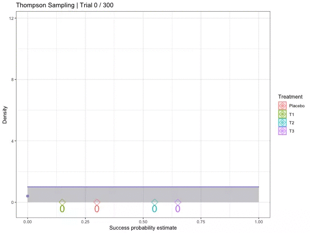
다중 팔 슬롯머신(Multi-Armed Bandit Problem)에서 탐험과 활용 사이의 딜레마를 해결하기 위한 휴리스틱 방법으로, 이 접근 방식의 목표는 과거의 관측과 어떤 기저 확률 분포를 바탕으로 최선의 행동을 선택하여 누적 보상을 최대화하는 것입니다.

[톰슨 샘플링의 구성 요소]

우도 함수 (Likelihood Function) $P(r\\|\theta, a, x)$: 이 함수는 파라미터 $\theta$, 행동 $a$, 컨텍스트 $x$가 주어졌을 때 보상 $r$을 받을 확률을 설명합니다.
파라미터 집합 (Parameter Set) $\Theta$: 이 집합은 보상의 분포를 정의하는 파라미터 $\theta$의 모든 가능한 값을 포함합니다.
사전 분포 (Prior Distribution) $P( ext)$: 이는 어떤 관측도 이루어지기 전에 파라미터 $\theta$의 분포에 대한 초기 신념입니다.
과거 관측 (Past Observations) $D = \{(x; a; r)\}$: 이는 이전 라운드에서 수집한 컨텍스트 $x$, 행동 $a$, 받은 보상 $r$로 구성된 역사적 데이터입니다.
사후 분포 (Posterior Distribution) $P( ext\\|D)$

이는 과거 관측 $D$가 주어졌을 때 파라미터 $\theta$에 대한 사후 분포입니다. 베이즈 정리(Bayes’ theorem)를 사용하여 다음과 같이 계산됩니다.

\[P( ext\\|D) \propto P(D\\|\theta) P( ext)\]

$P(D\\|\theta)$는 우도 함수입니다.

[톰슨 샘플링의 구현]

톰슨 샘플링은 다음의 절차로 구현됩니다.

각 라운드마다 파라미터 $\theta^*$를 사후 분포 $P( ext\\|D)$에서 샘플링합니다.
현재의 컨텍스트 $x$와 샘플링된 파라미터 $\theta^*$가 주어졌을 때 기대 보상 $\mathbb{E}[r\\|\theta^*, a, x]$를 최대화하는 행동 $a^*$를 선택합니다.

$a^* = \arg\max_{a \in \mathcal{A}} \mathbb{E}[r\\|\theta^*, a, x]$

선택한 행동 $a^*$를 실행하고, 해당 보상 $r$을 관측합니다.
관측한 데이터 $(x, a^*, r)$를 과거 관측 $D$에 추가하고 사후 분포 $P( ext\\|D)$를 갱신합니다.

톰슨 샘플링은 다중 팔 슬롯머신뿐만 아니라, 다양한 온라인 학습 문제에 널리 사용되는데, A/B 테스트, 온라인 광고, 그리고 분산 의사결정 문제에서의 가속 학습 등에 활용되며, 특히 실제 응용에서 사후 분포를 유지하고 샘플링하는 것이 부담 되는 경우 근사 샘플링 기법(Sampling Methods for Approximate Inference)과 결합하여 사용되기도 합니다.

Thompson Sampling with Approximate Inference

1 Introduction

Recent progress on Large Language Models (LLMs) is having a transformative effect not only in natural language processing but also more broadly in a range of AI applications (Radford et al., 2019; Chowdhery et al., 2022; Brown et al., 2020; Touvron et al., 2023; Bubeck et al., 2023; Schulman et al., 2022; OpenAI, 2023; Anthropic, 2023). A key ingredient in the roll-out of LLMs is the fine-tuning step, in which the models are brought into closer alignment with specific behavioral and normative goals. When no adequately fine-tuned, LLMs may exhibit undesirable and unpredictable behavior, including the fabrication of facts or the generation of biased and toxic content (Perez et al., 2022; Ganguli et al., 2022). The current approach towards mitigating such problems is to make use of reinforcement learning based on human assessments. In particular, Reinforcement Learning with Human Feedback (RLHF) proposes to use human assessments as a reward function from pairwise or multi-wise comparisons of model responses, and then fine-tune the language model based on the learned reward functions (Ziegler et al., 2019; Ouyang et al., 2022; Schulman et al., 2022).

Following on from a supervised learning stage, a typical RLHF protocol involves two main steps:

Reward learning: Sample prompts from a prompt dataset and generate multiple responses for the same prompt. Collect human preference data in the form of pairwise or multi-wise comparisons of different responses. Train a reward model based on the preference data.
Policy learning: Fine-tune the current LLM based on the learned reward model with reinforcement learning algorithms.

Although RLHF has been successful in practice (Bai et al., 2022; Ouyang et al., 2022; Dubois et al., 2023), it is not without flaws, and indeed the current reward training paradigm grapples with significant value-reward mismatches. There are two major issues with the current paradigm:

Reward overfitting: During the training of the reward model, it has been observed that the test cross-entropy loss of the reward model can deteriorate after one epoch of training Ouyang et al. (2022).
Reward overoptimization: When training the policy model to maximize the reward predicted by the learned model, it has been observed that the ground-truth reward can increase when the policy is close in KL divergence to the initial policy, but decrease with continued training (Gao et al., 2023).

In this paper, we investigate these issues in depth. We simplify the formulation of RLHF to a multi-armed bandit problem and reproduce the overfitting and overoptimization phenomena. We leverage theoretical insights in the bandit setting to design new algorithms that work well under practical fine-tuning scenarios.

1.1 Main Results

As our first contribution, we pinpoint the root cause of both reward overfitting and overoptimization. We show that it is the inadequacy of the cross-entropy loss for long-tailed preference datasets. As illustrated in Figure 1, even a simple 3-armed bandit problem can succumb to overfitting and overoptimization when faced with such imbalanced datasets. Consider a scenario where we have three arms with true rewards given by r⋆ 3 = 0, and the preference distribution is generated by the Bradley-Terry-Luce (BTL) model (Bradley and Terry, 1952), i.e. P(i ≻ j) = exp(r⋆ j). Suppose our preference dataset compares the first and second arms 1000 times but only compares the first and third arm once, and let n(i ≻ j) denote the number of times that arm i is preferred over arm j. The standar empirical cross-entropy loss used in the literature for learning the reward model (Ouyang et al., 2022; Zhu et al., 2023a) can be written as follows:

We know that the empirical values n(1 ≻ 2) and n(2 ≻ 1) concentrate around their means. However, we have with probability 0.73, n(1 ≻ 3) = 1 and n(3 ≻ 1) = 0, and with probability 0.27, n(1 ≻ 3) = 0 and n(3 ≻ 1) = 1. In either case, the minimizer of the empirical entropy loss will satisfy either ˆr1 − ˆr3 = −∞ or ˆr1 − ˆr3 = +∞. This introduces a huge effective noise when the coverage is imbalanced. Moreover, the limiting preference distribution is very different from the ground truth distribution, leading to reward overfitting. Furthermore, since there is 0.27 probability that ˆr1 − ˆr3 = −∞, we will take arm 3 as the optimal arm instead of arm 1. This causes reward overoptimization during the stage of policy learning since the final policy converges to the wrong arm with reward zero.

Figure 1. Illustration of the problem of the vanilla empirical cross-entropy minimization for learning the ground truth reward. With a small number of samples comparing arm 1 and 3, the minimization converges to a solution which assigns ˆr1 − ˆr3 = −∞ with constant probability. With the proposed Iterative Data Smoothing (IDS) algorithm, the estimator is able to recover the ground truth reward.

To mitigate these effects, we leverage the pessimism mechanism from bandit learning to analyze and design a new algorithm, Iterative Data Smoothing (IDS), that simultaneously addresses both reward overfitting and reward overoptimization. The algorithm design is straightforward: in each epoch, beyond updating the model with the data, we also adjust the data using the model. Theoretically, we investigate the two phenomena in the tabular bandit case. We show that the proposed method, as an alternative to the lower-confidence-bound-based algorithm (Jin et al., 2021; Xie et al., 2021; Rashidinejad et al., 2021; Zhu et al., 2023a), learns the ground truth distribution for pairs that are compared enough times, and ignores infrequently covered comparisons thereby mitigating issues introduced by long-tailed data. Empirically, we present experimental evidence that the proposed method improves reward training in both bandit and neural network settings.

RLHF and Preference-based Reinforcement Learning. RLHF, or Preference-based Reinforcement Learning (PbRL), has delivered significant empirical success in the fields of game playing, robot training, stock prediction, recommender systems, clinical trials and natural language processing (Novoseller et al., 2019; Sadigh et al., 2017; Christiano et al., 2017b; Kupcsik et al., 2018; Jain et al., 2013; Wirth et al., 2017; Knox and Stone, 2008; MacGlashan et al., 2017; Christiano et al., 2017a; Warnell et al., 2018; Brown et al., 2019; Shin et al., 2023; Ziegler et al., 2019; Stiennon et al., 2020; Wu et al., 2021; Nakano et al., 2021; Ouyang et al., 2022; Menick et al., 2022; Glaese et al., 2022; Gao et al., 2022; Bai et al., 2022; Ganguli et al., 2022; Ramamurthy et al., 2022). In the setting of the language models, there has been work exploring the efficient fine-tuning of the policy model (Snell et al., 2022; Song et al., 2023a; Yuan et al., 2023; Zhu et al., 2023b; Rafailov et al., 2023; Wu et al., 2023).

In the case of reward learning, Ouyang et al. (2022) notes that in general the reward can only be trained for one epoch in the RLHF pipeline, after which the test loss can go up. Gao et al. (2023) studies the scaling law of training the reward model, and notes that overoptimization is another problem in reward learning. To address the problem, Zhu et al. (2023a) propose a pessimism-based method that improves the policy trained from the reward model when the optimal reward lies in a linear family. It is observed in Song et al. (2023b) that the reward model tends to be identical regardless of whether the prompts are open-ended or closed-ended during the terminal phase of training, and they propose a prompt-dependent reward optimization scheme.

Another closely related topic is the problem of estimation and ranking from pairwise or K-wise comparisons. In the literature of dueling bandit, one compares two actions and aims to minimize regret based on pairwise comparisons (Yue et al., 2012; Zoghi et al., 2014b; Yue and Joachims, 2009, 2011; Saha and Krishnamurthy, 2022; Ghoshal and Saha, 2022; Saha and Gopalan, 2018a; Ailon et al., 2014; Zoghi et al., 2014a; Komiyama et al., 2015; Gajane et al., 2015; Saha and Gopalan, 2018b, 2019; Faury et al., 2020). Novoseller et al. (2019); Xu et al. (2020) analyze the sample complexity of dueling RL agents in the tabular case, which is extended to linear case and function approximation by the recent work of Pacchiano et al. (2021); Chen et al. (2022). Chatterji et al. (2022) studies a related setting where in each episode only binary feedback is received. Most of the theoretical work of learning from ranking focuses on regret minimization, while RLHF focuses more on the quality of the final policy.

Knowledge Distillation The literature of knowledge distillation focuses on transferring the knowledge from a teacher model to a student model (Hinton et al., 2015; Furlanello et al., 2018; Cho and Hariharan, 2019; Zhao et al., 2022; Romero et al., 2014; Yim et al., 2017; Huang and Wang, 2017; Park et al., 2019; Tian et al., 2019; Tung and Mori, 2019; Qiu et al., 2022; Cheng et al., 2020). It is observed in this literature that the soft labels produced by the teacher network can help train a better student network, even when the teacher and student network are of the same size and structure Hinton et al. (2015). Furlanello et al. (2018) present a method which iteratively trains a new student network after the teacher network achieves the smallest evaluation loss. Both our iterative data smoothing algorithm and these knowledge distillation methods learn from soft labels. However, iterative data smoothing iteratively updates the same model and data, while knowledge distillation method usually focuses on transferring knowledge from one model to the other.

2 Formulation

We begin with the notation that we use in the paper. Then we introduce the general formulation of RLHF, along with our simplification in the multi-armed bandit case.

Notations. We use calligraphic letters for sets, e.g., S and A. Given a set S, we write |S| to represent the cardinality of S. We use [K] to denote the set of integers from 1 to K. We use µ(a, a′) to denote the probability of comparing a and a′ in a preference dataset, and µ(a) = (cid:80) a′∈A µ(a, a′) to denote the probability of comparing a with any other arms. Similarly, we use n(a), n(a, a′) to denote the number of samples that compare a with any other arms, and the number of samples that compare a with a′, respectively. We use a1 ≻ a2 to denote the event that the a1 is more preferred compared to a2.

2.1 General Formulation of RLHF

The key components in RLHF consist of two steps: reward learning and policy learning. We briefly introduce the general formulation of RLHF below.

In the stage of reward learning, one collects a preference dataset based on a prompt dataset and responses to the prompts. According to the formulation of Zhu et al. (2023a), for the i-th sample, a state (prompt) si is first sampled from some prompt distribution ρ. Given the state si, M actions (responses) (a(1) ) are sampled from some joint distribution P(a(1), · · · , a(M) | si), Let σi : [M] (cid:55)→ [M] i be the output of the human labeller, which is a permutation function that denotes the ranking of the actions. Here σi(1) represents the most preferred action, and σi(M ) is the least preferred action. A common model for the distribution of σ under multi-ary comparisons is a Plackett-Luce model (Plackett, 1975; Luce, 2012).

where r⋆ : S × A (cid:55)→ R is the ground-truth reward for the response given the prompt. Moreover, the probability of observing the permutation σ is defined as1

When M = 2, this reduces to the pairwise comparison considered in the Bradley-Terry-Luce (BTL) model (Bradley and Terry, 1952), which is used in existing RLHF algorithms. In this case, the permutation σ can be reduced to a Bernoulli random variable, representing whether one action is preferred compared to the other. Concretely, for each queried state-actions pair (s, a, a′), we observe a sample c from a Bernoulli exp(rθ⋆ (s,a))+exp(rθ⋆ (s,a′)) . Based on the observed dataset, the cross-entropy distribution with parameter loss is minimized to estimate the ground-truth reward for the case of pairwise comparison. The minimizer of cross-entropy loss is the maximum likelihood estimator:

After learning the reward, we aim to learn the optimal policy under KL regularization with respect to

an initial policy π0 under some state (prompt) distribution ρ′.

2.2 RLHF in Multi-Armed Bandits

To understand the overfitting and overoptimization problems, we simplify the RLHF problem to consider a single-state multi-armed bandit formulation with pairwise comparisons. Instead of fitting a reward model and policy model with neural networks, we fit a tabular reward model in a K-armed bandit problem.

1In practice, one may introduce an extra temperature parameter σ and replace all r⋆ with r⋆/σ. Here we take σ = 1.

Consider a multi-armed bandit problem with K arms. Each arm has a deterministic ground-truth reward r⋆(k) ∈ R, k ∈ [K]. In this case, the policy becomes a distribution supported on the K arms π ∈ ∆([K]). The sampling process for general RLHF reduces to the following: we first sample two actions ai, a′ i from a joint distribution µ ∈ ∆([K] × [K]), and then observe a binary comparison variable yi following a distribution

Assume that we are given n samples, which are sampled i.i.d. from the above process. Let n(a, a′) be the total number of comparisons between actions a and a′ in the n samples. Let the resulting dataset be D = {ai, a′ i=1. The tasks in RLHF for multi-armed bandit setting can be simplified as:

Reward learning: Estimate true reward r⋆ with a proxy reward ˆr from the comparison dataset D.
Policy learning: Find a policy π ∈ ∆([K]) that maximizes the proxy reward under KL constraints.

In the next two sections, we discuss separately the reward learning phase and policy learning phase, along with the reasons behind overfitting and overoptimization.

2.3 Overfitting in Reward Learning

For reward learning, the commonly used maximum likelihood estimator is the estimator that minimizes empirical cross-entropy loss:

By definition, ˆrMLE is convergent point when we optimize the empirical cross entropy fully. Thus the population cross-entropy loss of ˆrMLE is an indicator for whether overfitting exists during reward training.

We define the population cross entropy loss as

For a fixed pairwise comparison distribution µ, it is known that the maximum likelihood estimator

ˆrMLE converges to the ground truth reward r⋆ as the number of samples n goes to infinity.

Theorem 2.1 (Consistency of MLE, see, e.g., Theorem 6.1.3. of Hogg et al. (2013)). Fix r⋆(K) = ˆr(K) = 0 for the uniqueness of the solution. For any fixed µ, and any given ground-truth reward r⋆, we have that ˆrMLE converges in probability to r⋆; i.e., for any ϵ > 0,

Here we view ˆrMLE and r⋆ as K-dimensional vectors.

The proof is deferred to Appendix D. This suggests that the overfitting phenomenon does not arise when we have an infinite number of samples. However, in the non-asymptotic regime when the comparison distribution µ may depend on n, one may not expect convergent result for MLE. We have the following theorem.

Theorem 2.2 (Reward overfitting of MLE in the non-asymptotic regime). Fix r⋆(a) = 1(a = 1) and ˆr(K) = 0 for uniqueness of the solution. For any fixed n > 500, there exists some 3-armed bandit problem such that with probability at least 0.09,

for any arbitrarily large C.

LCE(ˆrMLE) − LCE(r⋆) ≥ C

The proof is deferred to Appendix E. Below we provide a intuitive explanation. The constructed hard instance is a bandit where r⋆(a) = 1(a = 1). For any fixed n, we set µ(1, 2) = 1 − 1/n, µ(1, 3) = 1/n.

In this hard instance, there is constant probability that arm 3 is only compared with 1 once. And with constant probability, the observed comparison result between arm 1 and arm 3 will be different from the ground truth. The MLE will assign r(3) = +∞ since the maximizer of log(exp(x)/(1 + exp(x))) is infinity when x is not bounded. Thus when optimizing the empirical cross entropy fully, the maximum likelihood estimator will result in a large population cross-entropy loss. We also validate this phenomenon in Section 4.1 with simulated experiments.

This lower bound instance simulates the high-dimensional regime where the number of samples is comparable to the dimension, and the data coverage is unbalanced across dimensions. One can also extend the lower bound to more than 3 arms, where the probability of the loss being arbitrarily large will be increased to close to 1 instead of a small constant.

2.4 Overoptimization in Policy Learning

After obtaining the estimated reward function ˆr, we optimize the policy π ∈ ∆([K]) to maximize the estimated reward. In RLHF, one starts from an initial (reference) policy π0, and optimizes the new policy π to maximize the estimated reward ˆr under some constraint in KL divergence between π and π0. It is observed in Gao et al. (2022) that as we continue optimizing the policy to maximize the estimated reward, the true reward of the policy will first increase then decrease, exhibiting the reward overoptimization phenomenon.

Consider the following policy optimization problem for a given reward model ˆr:

Assuming that the policy gradient method converges to the optimal policy for the above policy optimization problem, which has a closed-form solution:

In the tabular case, we can derive a closed form solution for how the KL divergence and ground-truth reward change with respect to λ, thus completely characterizing the reward-KL tradeoff. We compute the KL divergence and ground-truth reward of the policy as

The above equation provides a precise characterization of how the mismatch between ˆr and r⋆ leads to the overoptimization phenomenon, which can be validated from the experiments in Section 4. To simplify the analysis and provide better intuition, we focus on the case when λ → ∞, i.e., when the optimal policy selects the best empirical arm without considering the KL constraint. In this case, the final policy reduces to the empirical best arm, π∞(a) = 1(a = arg maxa′ ˆr(a′)).

By definition, π∞ is the convergent policy when we keep loosening the KL divergence constraint in Equation (2). Thus the performance of π∞ is a good indicator of whether overoptimization exists during policy training. We thus define a notion fo sub-optimality to characterize the performance gap between the convergent policy and the optimal policy:

We know from Theorem 2.1 that, asymptotically, the MLE for reward ˆrMLE converges to the ground truth reward r⋆. As a direct result, when using the MLE as reward, the sub-optimality of the policy π∞ also converges to zero with an infinite number of samples.

However, as a corollary of Theorem 2.2 and a direct consequence of reward overfitting, π∞ may have large sub-optimality in the non-asymptotic regime when trained from ˆrMLE.

Corollary 2.3 (Reward overoptimization of MLE in the non-asymptotic regime). Fix r⋆(a) = 1(a = 1). For any fixed n, there exists some 3-armed bandit problem such that with probability at least 0.09, SubOpt(ˆπ∞) ≥ 1.

The proof is deferred to Appendix F. This suggests that ˆrMLE also leads to the reward overoptimization phenomenon in the non-asymptotic regime. In Section 4, we conduct simulation in the exact same setting to verify the theoretical results.

3 Methods: Pessimistic MLE and Iterative Data Smoothing

The problem of overfitting and overoptimization calls for a design of better and practical reward learning algorithm that helps mitigate both issues. We first discuss the pessimistic MLE algorithm in Zhu et al. (2023a), which is shown to converge to a policy with vanishing sub-optimality under good coverage assumption.

3.1 Pessimistic MLE

In the tabular case, the pessimistic MLE corrects the original MLE by subtracting a confidence interval. Precisely, we have

where n is the total number of samples and λ = ∥(L + ϵI)−1/2 ∥2 is the norm of the j-th column of the matrix (L + ϵI)−1/2, where L is the matrix that satisfies La,a = n(a)/n, La,a′ = −n(a, a′)/n, ∀a ̸= a′, and ϵ is a small constant. Intuitively, for those arms that are compared fewer times, we are more uncertain about their ground-truth reward value. Pessimistic MLE penalizes these arms by directly subtracting the length of lower confidence interval of their reward, making sure that the arms that are less often compared will be less likely to be chosen. It is shown in Zhu et al. (2023a) that the sub-optimality of the policy optimizing ˆrPE converges to zero under the following two conditions:

The expected number of times that one compares optimal arm (or the expert arm to be compared with in the definition of sub-optimality) is lower bounded by some positive constant µ(a⋆) ≥ C.
The parameterized reward family lies in a bounded space |ˆr(a)| ≤ B, ∀a ∈ [K].

This indicates that pessimistic MLE can help mitigate the reward overoptimization phenomenon. However, for real-world reward training paradigm, the neural network parameterized reward family may not be bounded. Furthermore, estimating the exact confidence interval for a neural-network parameterized model can be hard and costly. This prevents the practical use of pessimistic MLE, and calls for new methods that can potentially go beyond these conditions and apply to neural networks.

3.2 Iterative Data Smoothing

We propose a new algorithm, Iterative Data Smoothing (IDS), that shares similar insights as pessimistic MLE. Intuitively, pessimistic MLE helps mitigate the reward overoptimization issue by reducing the estimated reward for less seen arms. In IDS, we achieve this by updating the label of the data we train on.

Algorithm 1 Iterative Data Smoothing (D, θ0, α, β)

Input: The pairwise comparison dataset D = {ai, a′ {rθ : A (cid:55)→ R

θ ∈ Θ} with initialization θ0 ∈ Θ. Two step sizes α, β. An empirical loss function

As is shown in Algorithm 1, we initialize yi,0 as the labels for the samples yi. In the t-th epoch, we first update the model using the current comparison dataset with labels {yi,t}n i=1. After the model is updated, we also update the data using the model by predicting the probability P(yi = 1) for each comparison (ai, a′ i) using the current reward estimate ˆrθt. We update each label yi,t as a weighted combination of its previous value and the new predicted probability.

Intuitively, yi,t represents a proxy of the confidence level of labels predicted by interim model checkpoints. The idea is that as the model progresses through multiple epochs of training, it will bring larger change to rewards for frequently observed samples whose representation is covered well in the dataset. Meanwhile, for seldom-seen samples, the model will make minimal adjustments to the reward.

3.2.1 Benefit of one-step gradient descent

Before we analyze the IDS algorithm, we first discuss why training for one to two epochs in the traditional reward learning approach works well (Ouyang et al., 2022). We provide the following analysis of the one-step gradient update for the reward model. The proof is deferred to Appendix G.

Theorem 3.1. Consider the same multi-armed bandit setting where the reward is initialized equally for all K arms. Then after one-step gradient descent, one has

∀a, a′ ∈ [K], ˆr(a) − ˆr(a′) = α · (n+(a) − n−(a) − (n+(a′) − n−(a′))),

where n+(a), n−(a) refers to the total number of times that a is preferred and not preferred, respectively.

Remark 3.2. The result shows that why early stopping in the traditional reward learning works well in a simple setting. After one gradient step, the empirical best arm becomes the the arm whose absolute winning time is the largest. This can be viewed as another criterion besides pessimism that balances both the time of comparisons and the time of being chosen as the preferred arm. When the arm a is only compared few times, the difference n+(a) − n−(a) will be bounded by the total number of comparisons, which will be smaller than those that have been compared much more times. Thus the reward model will penalize those arms seen less. After updating the label with the model prediction, the label of less seen samples will be closer to zero, thus getting implicitly penalized.

3.2.2 Benefit of iterative data smoothing

Due to under-optimization, the estimator from a one-step gradient update might still be far from the ground-truth reward. We provide an analysis here why IDS can be better. Consider any two arms a, a′ with n(a, a′) observations among n total observations. By computing the gradient, we can write the IDS algorithm as

where we define ˆµ(a ≻ a′) = n(a ≻ a′)/n(a, a′). One can see that the effective step size for updating ˆr is α · n(a, a′)/n, while the effective step size for updating y is β. Assume that we choose α, β, l, m such that

Consider the following two scales:

α · l/n ≪ β ≪ α · m/n.

When there are sufficient observations, n(a, a′) ≥ m, we know that β ≪ α · n(a, a′)/n. In this case, the update step size of yt is much slower than ˆrt. One can approximately take yt ≈ 0 or 1 as unchanged during the update. Furthermore, since n(a, a′) ≥ m is large enough, ˆµ concentrates around the ground truth µ. In this case, one can see that the reward converges to the ground truth reward ˆrt → r⋆.
When the number of observations is not large, i.e., n(a, a′) ≤ l, we know that α · l/n ≪ β. In this case, the update of ˆr is much slower than yt. When the ˆr0 are initialized to be zero, yt will first converge to 1/2, leading to ˆrt(a) ≈ ˆrt(a′) when t is large.

To formalize the above argument, we consider the following differential equations:

Here d represents the difference of reward between two arms a, a′, and µ represents the empirical frequency ˆµ(a ≻ a′). Let the initialization be d(0) = 0, y(0) = 1. We have the following theorem.

Theorem 3.3. The differential equations in Equation (5) have one unique stationary point d(t) = 0, y(t) = 1 2 . On the other hand, for any α, β, n, T with βT ≤ ϵ ≪ 1 ≪ αnT , one has

The proof is deferred to Appendix H. Note that the above argument only proves convergence to the empirical measure µ. One can combine standard concentration argument to prove the convergence to the ground truth probability. The result shows that when choosing α, β carefully, for the pair of arms with a large number of comparisons, the difference of reward will be close to the ground truth during the process of training. As a concrete example, by taking α = n−1/2, β = n−1T −2, ϵ = βT , we have

One can see that for those pairs of comparisons with a large sample size n, the estimated probability is close to the ground truth probability. On the other hand, for those pairs that are compared less often, the difference d(t) is updated less frequently and remains close to the initialized values. Thus the algorithm implicitly penalizes the less frequently seen pairs, while still estimating the commonly seen pairs accurately.

In summary, the IDS algorithm enjoys several benefits:

For a sufficient number of observations, the estimated reward approximately converges to the ground truth reward; while for an insufficient number of observations, the estimated reward remains largely unchanged at the initialization. Thus the reward model penalizes the less observed arms with higher uncertainty.
It is easy to combine with neural networks, allowing arbitrary parametrization of the reward model.
It utilizes the soft labels starting from the second epoch, which can be more effective than hard labels according to the literature on knowledge distillation (Hinton et al., 2015; Zhao and Zhu, 2023).

We also present an alternative formulation of IDS in Appendix B.

Figure 2: Comparisons of the three methods in the multi-armed bandit setting.

4 Experiments

In this section, we present the results of experiments with both multi-armed bandits and neural networks.

4.1 Multi-Armed Bandit

In the bandit setting, we focus on the hard example constructed in Theorem 2.2. We take total samples n = 60 and the number of arms K as 10 and 20. We compare the performance of the vanilla MLE, pessimistic MLE and IDS in both the reward learning phase and the policy learning phase.

In the reward learning phase, we run stochastic gradient descent with learning rate 0.01 on the reward model for multiple epochs and monitor how the loss changes with respect to the number of training epochs. For pessimistic MLE, we subtract the confidence level in the reward according to Equation (4). For IDS, we take the two step sizes as α = 0.01, β = 0.001. As is shown in left part of Figure 2, both MLE and pessimistic MLE suffer from reward overfitting, while the test cross-entropy loss for the IDS algorithm continues to decrease until convergence. Since the training loss changes with the updated labels, we plot the population cross-entropy loss which is averaged over all pairs of comparisons.

In the right part of the figure, we plot the KL-reward tradeoff when training a policy based on the learned reward. We vary the choice of λ in Equation (3) to derive the optimal policy under diverse levels of KL constraint, where we take the reference policy π0 as the uniform policy. One can see that IDS is able to converge to the optimal reward when KL is large, while both MLE and pessimistic MLE suffer from overoptimization.

We remark here that the reason pessimistic MLE suffers from both overfitting and overoptimization might be due to the design of unbounded reward in the multi-armed bandit case. When the reward family is bounded, pessimistic MLE is also guaranteed to mitigate the overoptimization issue. Furthermore, we only run one random seed for this setting to keep the plot clean since the KL-reward trade-off heavily depends on the observed samples.

4.2 Neural Network

We also conduct experiments with neural networks. We use the human-labeled Helpfulness and Harmlessnes (HH) dataset from Bai et al. (2022).2 We take Dahoas/pythia-125M-static-sft3 as the policy model with three different reward models of size 125M, 1B and 3B. When training reward model, we take a supervised fine-tuned language model, remove the last layer and replace it with a linear layer. When fine-tuning the language model, we use the proximal policy optimization (PPO) algorithm (Schulman et al., 2017).

We take a fully-trained 6B reward model Dahoas/gptj-rm-static trained from the same dataset based on EleutherAI/gpt-j-6b as the ground truth. We use the model to label the comparison samples using the BTL model (Bradley and Terry, 1952). And we train the 125M, 1B and 3B reward model with the new labeled comparison samples. The reward training results are shown in Figure 3. One can see that the MLE begins to overfit after 1-2 epochs, while the loss of the IDS algorithm continues to decrease stably until convergence.

For both MLE and IDS algortihms, we take the reward with the smallest evaluation loss and optimize a policy against the selected reward model. We compare results for policy learning as shown in Figure 4. One can see that MLE suffers from reward overoptimization with few thousand steps, while the ground truth reward continues to grow when using our IDS algorithm. We select step sizes α = 10−5 and β = 0.7 for all experiments. We observe that larger model leads to more improvement after one epoch, potentially due to more accurate estimation of the labels. We provide more details of the experiment along with the experiments on a different dataset, TLDR, in Appendix C.

In the implementation, we find that it is helpful to restore the best checkpoint at the end of each epoch. This is due to that an inappropriate label {yi}n i=1 at certain epoch may hurt the performance of the model. To prevent overfitting to the test set, we choose a large validation and test dataset, and we select the best checkpoint according to the smallest loss in the validation set, and plot the loss on the test set. During the whole training procedure including checkpoint restoration, we do not use any of the sample in the test set.

2 https://huggingface.co/datasets/Dahoas/static-hh

3 https://huggingface.co/Dahoas/pythia-125M-static-sft

Figure 3: Comparisons of MLE and IDS when the reward is parameterized by a neural network.

Figure 4: Comparison of MLE and IDS for policy learning

5 Conclusions

We have presented analyses and methodology aimed at resolving the problems of overfitting and overoptimization in reward training for RLHF. We show that our proposed algorithm, IDS, helps mitigate these two issues in both the multi-armed bandit and neural network settings. Note that while we identify the underlying source of reward overfitting and overoptimization as the variance of the human preference data, it is also possible that bias also contributes to these phenomena. In future work, plan to pursue further formal theoretical analysis of the IDS algorithm, and explore potential applications beyond reward training in the generic domains of classification and prediction.

post contain ""

No matching posts found containing ""

Iterative Data Smoothing**

Iterative Data Smoothing**

Iterative Data Smoothing**

Iterative Data Smoothing: Mitigating Reward Overfitting and Overoptimization in RLHF

TL;DR

1 Introduction

1.1 Main Results

2 Formulation

2.1 General Formulation of RLHF

2.2 RLHF in Multi-Armed Bandits

2.3 Overfitting in Reward Learning

2.4 Overoptimization in Policy Learning

3 Methods: Pessimistic MLE and Iterative Data Smoothing

3.1 Pessimistic MLE

3.2 Iterative Data Smoothing

3.2.1 Benefit of one-step gradient descent

3.2.2 Benefit of iterative data smoothing

4 Experiments

4.1 Multi-Armed Bandit

4.2 Neural Network

5 Conclusions

post contain ""

No matching posts found containing ""

Recent Posts

Most Likes

Most Views

Share Your Feedback 🏝️

Iterative Data Smoothing**

Iterative Data Smoothing**

Iterative Data Smoothing: Mitigating Reward Overfitting and Overoptimization in RLHF

TL;DR

1 Introduction

1.1 Main Results

1.2 Related Work

2 Formulation

2.1 General Formulation of RLHF

2.2 RLHF in Multi-Armed Bandits

2.3 Overfitting in Reward Learning

2.4 Overoptimization in Policy Learning

3 Methods: Pessimistic MLE and Iterative Data Smoothing

3.1 Pessimistic MLE

3.2 Iterative Data Smoothing

3.2.1 Benefit of one-step gradient descent

3.2.2 Benefit of iterative data smoothing

4 Experiments

4.1 Multi-Armed Bandit

4.2 Neural Network

5 Conclusions

post contain ""

No matching posts found containing ""

Recent Posts

Most Likes

Most Views