PL | Contrastive Preference Learning*

• Related Project: Private
• Category: Paper Review
• Date: 2024-01-13

Contrastive Preference Learning: Learning from Human Feedback without RL

• url: https://arxiv.org/abs/2310.13639
• pdf: https://arxiv.org/pdf/2310.13639
• github: https://github.com/jhejna/cpl
• abstract: Reinforcement Learning from Human Feedback (RLHF) has emerged as a popular paradigm for aligning models with human intent. Typically RLHF algorithms operate in two phases: first, use human preferences to learn a reward function and second, align the model by optimizing the learned reward via reinforcement learning (RL). This paradigm assumes that human preferences are distributed according to reward, but recent work suggests that they instead follow the regret under the user’s optimal policy. Thus, learning a reward function from feedback is not only based on a flawed assumption of human preference, but also leads to unwieldy optimization challenges that stem from policy gradients or bootstrapping in the RL phase. Because of these optimization challenges, contemporary RLHF methods restrict themselves to contextual bandit settings (e.g., as in large language models) or limit observation dimensionality (e.g., state-based robotics). We overcome these limitations by introducing a new family of algorithms for optimizing behavior from human feedback using the regret-based model of human preferences. Using the principle of maximum entropy, we derive Contrastive Preference Learning (CPL), an algorithm for learning optimal policies from preferences without learning reward functions, circumventing the need for RL. CPL is fully off-policy, uses only a simple contrastive objective, and can be applied to arbitrary MDPs. This enables CPL to elegantly scale to high-dimensional and sequential RLHF problems while being simpler than prior methods.

Contents

• Contrastive Preference Learning: Learning from Human Feedback without RL
  • TL;DR
  • Contrastive Preference Learning (CPL)
  • 1 INTRODUCTION
  • 2 PRELIMINARIES
  • 3 CONTRASTIVE PREFERENCE LEARNING
    • 3.1 FROM OPTIMAL ADVANTAGE TO OPTIMAL POLICY
    • 3.2 PRACTICAL CONSIDERATIONS
  • 4 EXPERIMENTS
    • 4.1 HOW DOES CPL PERFORM?
  • 5 RELATED WORK
  • 6 DISCUSSION

TL;DR

Contrastive Preference Learning(이하 “CPL”)은 복잡한 강화학습 과정 없이 직접적으로 선호도 데이터로부터 최적 policy를 학습할 수 있는 방법을 제시하여 기존 RLHF 방법들의 한계를 개선하는 동시에, 지도 학습의 목적함수의 변형을 통해 (전통적인 강화학습과는 달리) 직접적으로 선호도 데이터만으로 policy을 학습할 수 있기 때문에 확장가능하며, 효율적이라고 언급합니다.

CPL은 전통적인 강화학습 프로세스와 달리 보상 함수를 직접 학습하는 대신 선호도 모델을 기반으로 최적의 policy을 추출하는 방법이며 다음과 같은 요소를 특징으로 함.

1. CPL은 전통적인 보상 함수가 아니라, 선행 연구(Knox et al., 2022)를 인용해 사용자의 후회(regret, 그 외 Iterative Data Smoothing 혹은 다양한 논문의 참고자료 참조)를 기반으로 한 선호도 모델을 사용한다는 것을 인용. (일반적인 강화학습에서 보상 함수를 대체하는 방법 중 하나)
2. 최대 엔트로피(Maximum Entropy)를 통해 보상 함수와 policy 사이의 일대일 대응 관계를 설정 (시스템의 불확실성을 최대화하는 방식으로 최적의 결정을 위한 정보적 접근 방법 中 하나)
3. 최적의 보상 함수 \(A^*(s,a)\)와 온도 파라미터 \(\alpha\)를 사용하여 보상 함수 \(r(s, a)\)를 policy \(\pi^*(a\\|s)\)의 로그-우도와 연결하여, 선호도 데이터 기반 policy 최적화를 수행
4. 지도 학습 목적함수(CPL의 목적함수 변형 부분 참고)를 사용하여 최적의 policy을 학습하므로, traditional한 강화학습과 달리 직접적으로 선호도 데이터만을 사용하여 policy을 학습하므로 효율적이라고 주장.
5. 결론적으로 CPL의 목적함수는 로그 확률의 가중 합을 사용하여 선호되는 행동과 그렇지 않은 행동을 비교하는 contrastive 목적함수 형태로 나타내며, 이 목적함수는 선호도 데이터에서 추출된 정보를 최대화하여 최적의 policy을 학습하는 것에 중점을 둠. (Section 3.2 참고)

이런 요인들로 다양한 유형의 마르코프 결정 프로세스(MDP)에 적용 가능하며, RLHF의 한계를 극복하고, 용이하고 확장가능한 방법으로 모델을 더 효율적으로 학습할 수 있다고 주장

연구 배경

1. 대규모 사전 훈련 모델(large pretrained models)이 발전함에 따라 이를 휴먼의 선호도와 일치시키는 것이 중요한 연구 주제가 되었고, 이런 alignment 문제는 대규모 데이터셋에 최적이 아닌 행동들이 포함되어 있을 때 특히 어려울 수 있음.
2. 휴먼 피드백을 통한 강화학습(Reinforcement Learning from Human Feedback, RLHF)이 최근 human preference에 사용되고 있음.

RLHF가 최근 인기가 급상승했지만, 휴먼 선호(human preference)도로부터 policy을 학습하는 것은 PbRL(Preference-based RL)이라고 하는 연구 주제였음.

[기존 RLHF의 문제점]

1. 대부분의 RLHF 알고리즘은 통상적으로 다음 두 단계로 구성
   • a. 사용자 선호도 데이터로부터 보상 모델(reward model)을 학습하고,
   • b. 강화학습(RL) 알고리즘을 사용하여 이 보상 모델을 최적화

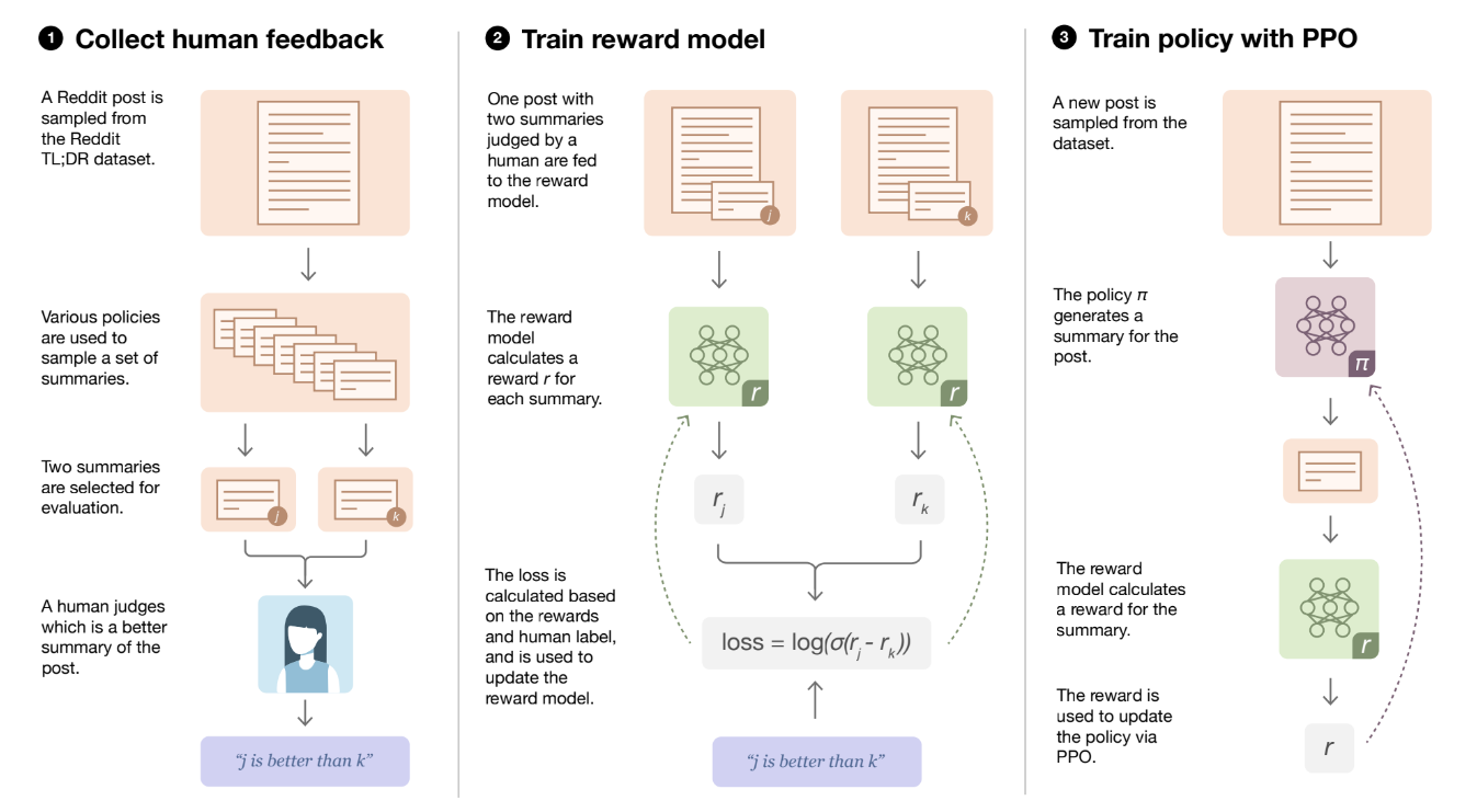   *출처: Learning to summarize from human feedback (Stiennon et al., 2022)

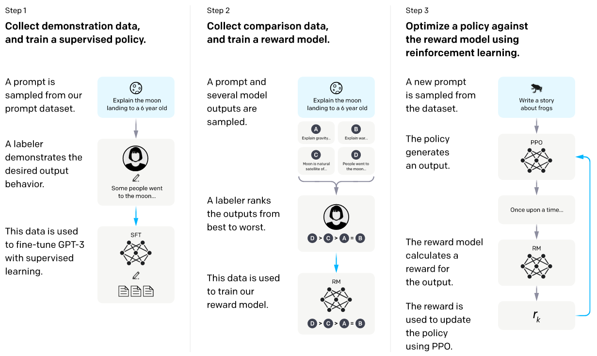   *출처: Open AI

2. 그러나 저자는 다음과 같은 이유로 기존 RLHF 패러다임 가정에 한계가 있다고 주장
   • (1) 휴먼의 선호도(HF, Human Feedback = Human Preference)가 각 행동 세그먼트의 discounted rewards의 합에 따라 분포된다고 가정해야 하나 이는 실제와 다를 수 있으며,
   • (2) 최근 연구(Knox et al., 2022)에 따르면, 휴먼은 최적 policy(optimal policy)에 대한 후회(regret)를 기반으로 선호도를 제공함. (보상을 받을 더 나은 답변이 아닌 상대적으로 더 나쁜 답변을 선택하는 것이 쉬우므로, Meta의 경우 리커드^{Likert scale} 7점 척도 사용, 그 외 5점 척도를 사용하기도 하지만, DPO의 경우 이지선다로 빠르고 많이 선별할 수 있음.)
3. 또한, RL 알고리즘은 다음과 같은 최적화 문제를 갖고 있음.
   • 시간적 신용 할당(temporal credit assignment)의 어려움 ^{[참고자료 1]}
   • Policy 그래디언트의 높은 분산 ^{[참고자료 2]}
   • 근사 동적 프로그래밍(approximate dynamic programming)의 불안정성 ^{[참고자료 3]}

Contrastive Preference Learning (CPL)

위 내용을 바탕으로, CPL은 기존 RLHF 방법들의 한계를 극복하고 더 효율적이고 확장 가능한 학습 방법을 제시함.

저자는 CPL이 복잡한 RL 과정을 거치지 않고, 다음과 같이 직접적으로 선호도 데이터에서 최적 policy를 학습할 수 있다고 주장함.

1. CPL은 보상 함수 대신 후회(regret)를 기반으로 한 선호도 모델을 사용
2. 최대 엔트로피(Maximum Entropy) 원리를 적용하여 보상 함수(advantage function)와 정책(policy) 사이의 일대일 대응 관계를 통한 변형
3. 위 2를 통해, 지도 학습 목적함수를 유도하여 최적 policy를 학습하도록 변형
4. 최대 엔트로피 RL^{[참고자료 4]}에서는 다음 관계가 성립하는데, \(\int e^{A^*(s,a)/\alpha} da = 1\)
   \((A^*(s,a)\)는 최적 보상 함수^{[참고자료 5]}, $\alpha$는 온도 파라미터)

5. 이로부터 다음 관계를 유도할 수 있으며,

   \[r(s, a) = \alpha \log \pi^*(a \\| s)\]

   (\(r(s,a)\)는 보상 함수, $\pi^*(a|s)$는 최적 policy)

6. 위 유도식을 선호도 모델을 policy $\pi^*$에 대한 식으로 표현할 수 있으므로, 결론적으로 CPL의 목적함수를 다음과 같이 정의함.

CPL의 목적함수 (Section 3.2 참고)

위 식에서 ($\sigma^+$와 $\sigma^-$는 각각 선호되는 행동 세그먼트와 선호되지 않는 행동 세그먼트를 의미함)

상기 식은 본 논문의 핵심으로 강화 학습(中 Policy Optimization, PO)과 관련된 손실 함수 \(LCPL(\pi_\theta, D_{\text{pref}})\)를 나타내며, policy의 성능을 측정하기 위해 두 경로(trajectory) \(\tau^+\)와 \(\tau^-\)의 확률을 비교합니다. 이 손실 함수는 주어진 선호 데이터셋에서 두 경로의 policy 확률을 비교하여 모델이 더 선호되는 경로를 얼마나 잘 예측하는지를 측정하고, 각 경로의 확률은 policy의 로그 확률을 시간에 따른 discount factor를 사용하여 합산한 후 지수화하여 계산됩니다.

CPL의 목적함수 항별로 살펴보기

1. 손실 함수 \(LCPL(\pi_\theta, D_{\text{pref}})\)

손실 함수 \(LCPL(\pi_\theta, D_{\text{pref}})\)는 두 경로의 policy 확률을 비교하는 로그 우도(log-likelihood)를 의미하며, policy가 두 경로 중 선호되는 경로를 얼마나 잘 예측하는지 평가합니다.

2. 기대값 \(\mathbb{E}_{(\tau^+, \tau^-) \sim D_{\text{pref}}} [ \cdot ]\)

이 항은 두 경로 \((\tau^+, \tau^-)\)의 쌍에 대해 데이터셋 \(D_{\text{pref}}\)에서 샘플링된 기대값을 의미하며, \(D_{\text{pref}}\)는 선호 데이터셋(preference dataset)으로, 사용자 또는 시스템이 선호하는 경로와 그렇지 않은 경로의 쌍을 포함합니다. 위 식에서 기대값을 취하는 이유는 모델이 다양한 샘플에 대해 일반화되도록 하기 위함입니다.

3. 경로 \(\tau^+\)와 \(\tau^-\)

• \(\tau^+ = \{(s_t^+, a_t^+)\}_{t=0}^{T}\): “선호되는 경로(trajectory)”로 상태 \(s_t^+\)와 행동 \(a_t^+\)의 시퀀스로 구성
• \(\tau^- = \{(s_t^-, a_t^-)\}_{t=0}^{T}\): “선호되지 않는 경로”로 상태 \(s_t^-\)와 행동 \(a_t^-\)의 시퀀스로 구성

4. \(\pi_\theta(a_t \\| s_t)\)

정책(policy) \(\pi_\theta(a_t \\| s_t)\)는 주어진 상태 \(s_t\)에서 행동 \(a_t\)를 선택할 확률 분포를 나타냅니다. \(\theta\)는 policy의 파라미터를 의미합니다. 이 식은 주어진 상태에서 특정 행동을 선택할 확률을 나타내므로, policy의 성능을 평가하는 데 사용됩니다.

5. Discount Factor \(\gamma^t\)

Discount Factor는 미래의 보상을 얼마나 중요하게 여길지를 결정하고 \(\gamma\)는 시간 \(t\)에 따른 보상의 중요도를 조절하며, \(0 \leq \gamma \leq 1\)의 값을 가집니다. 합니다. \(\gamma^t\)는 시간 \(t\)에서의 보상을 할인한 뒤 합산하게 됩니다.

6. 지수 함수와 로그 함수

6.1. 지수 함수 \(\exp(\cdot)\)

policy의 로그 확률에 지수 함수를 취한 것은 그 확률 값을 더해주는 역할을 합니다. 예를 들어, \(\exp\left(\sum_t \gamma^t \log \pi_\theta(a_t \\| s_t)\right)\)는 시간 \(t\)에 걸쳐 할인된 policy 로그 확률의 합을 지수화한 값으로, policy의 전체 경로 확률을 계산합니다.

6.2. 로그 함수 \(\log(\cdot)\)

이 식의 외부에 있는 로그 함수는 확률 비율의 로그를 취함으로써 손실을 계산한 뒤, 경로 \(\tau^+\)가 \(\tau^-\)보다 더 선호될 확률을 비교하여 평가합니다.

7. 분수 내부의 식

분수 내부의 식은 두 경로의 policy 확률을 비교하면서 선호되는 경로 \(\tau^+\)의 확률이 두 경로 \(\tau^+\)와 \(\tau^-\)의 확률 합의 비율을 나타내서 모델이 선호도를 얼마나 잘 학습하는지 평가합니다.

CPL의 목적함수의 장점(논문의 주장)

• 지도 학습만큼이나 잘 확장되며,
• 완전히 off-policy이므로
• 임의의 마르코프 결정 프로세스(MDP)에 적용 가능

추가로 저자가 RLHF의 문제로 지적하는 RL 알고리즘은 다음과 같은 최적화 문제를 살펴보면 다음 섹션을 참조 (본 논문의 Preliminaries 섹션 참조, 부연 설명)

[기본 개념]

• 상태가치 함수

  상태가치 함수 \(V^\pi(s)\)는 policy \(\pi\)에 따라 상태 \(s\)에서 시작했을 때의 기대 누적 보상

  \[V^\pi(s) = \mathbb{E}_\pi[G_t \mid S_t = s]\]
  • \(\mathbb{E}_\pi\): policy \(\pi\)에 따른 기대값
  • \(S_t = s\): 시간 \(t\)에서의 상태가 \(s\)인 경우

• 행동가치 함수

  행동가치 함수 \(Q^\pi(s, a)\)는 policy \(\pi\)에 따라 상태 \(s\)에서 행동 \(a\)를 취했을 때의 기대 누적 보상

  \[Q^\pi(s, a) = \mathbb{E}_\pi[G_t \mid S_t = s, A_t = a]\]
  • \(A_t = a\): 시간 \(t\)에서의 행동이 \(a\)인 경우

• 보상 함수

  보상 함수 \(A^\pi(s, a)\)는 특정 행동의 상대적 가치를 나타내며, 주어진 상태에서 특정 행동을 취하는 것이 얼마나 좋은지 나타내는 척도로 사용

  \[A^\pi(s, a) = Q^\pi(s, a) - V^\pi(s)\]
  • \(Q^\pi(s, a)\): 상태 \(s\)에서 행동 \(a\)를 취했을 때의 기대 누적 보상
  • \(V^\pi(s)\): 상태 \(s\)에서의 기대 누적 보상

[참고자료 1]

RL 알고리즘의 최적화의 한계 (1) - Policy 그래디언트의 높은 분산

• Policy 그래디언트의 높은 분산 문제

  Policy 그래디언트 방법은 다음과 같은 목적함수를 최대화하는데,

  \[J( ext) = \mathbb{E}_{\pi_\theta}[\sum_{t=0}^{\infty} \gamma^t r_t]\]

  이 때, 그래디언트는 다음과 같이 계산되며,

  \[\nabla_\theta J( ext) = \mathbb{E}_{\pi_\theta}[\sum_{t=0}^{\infty} \nabla_\theta \log \pi_\theta(a_t\\|s_t) Q^{\pi_\theta}(s_t, a_t)]\]

  이 추정치가 높은 분산을 가질 가능성이 있으므로 학습을 불안정하게 만드는 원인 중 하나로 알려져있음.

[참고자료 2]

RL 알고리즘의 최적화의 한계 (2) - Temporal credit assignment의 어려움

• 시간적 신용 할당 문제 다음과 같은 벨만 방정식은 복잡한 환경에서 “정확히 해결”하는 것이 어려우며, 장기적인 결과에 대한 각 행동의 시간적 기여도를 “정확히 평가”하는 것은 어려운 과제임.

  벨만 방정식 \(Q^*(s,a) = r(s,a) + \gamma \mathbb{E}_{s' \sim P(s'\\|s,a)}[\max_{a'} Q^*(s',a')]\)

벨만 방정식의 근사 오류

벨만 방정식은 강화학습에서 최적의 policy를 찾기 위해 사용되는데, 방정식은 주어진 상태 \(s\)와 행동 \(a\)에 대해 최적의 행동가치 함수 \(Q^*\)를 계산함. 하기 수식에서 \(Q^*(s,a)\)는 상태 \(s\)에서 행동 \(a\)를 선택했을 때 기대할 수 있는 미래 보상의 총합을 의미함.

• \(r(s,a)\): 상태 \(s\)에서 행동 \(a\)를 취했을 때 즉시 받는 보상
• \(\gamma\): discount factor로 미래 보상의 현재 가치 조정, 통상적으로 (0, 1)
• \(\mathbb{E}_{s' \sim P(s'\\|s,a)}\): 상태 \(s\)에서 행동 \(a\)를 취한 후에 도달할 가능성이 있는 모든 후속 상태 \(s'\)에 대한 기대값
• \(\max_{a'} Q^*(s',a')\): 후속 상태 \(s'\)에서 가능한 모든 행동 \(a'\)에 대해 \(Q^*\) 값을 최대화하는 행동 선택

벨만 방정식을 사용하여 각 상태와 행동의 기여도를 계산하는 것은 다음과 같은 현실적인 문제로 인하여 근사하게 되고, 필연적으로 근사오류가 발생하게 되는데, 저자는 이런 잠재적 추정 오류를 갖고있는 RLHF의 보다 CPL의 방법이 더 우수하다고 주장

• (문제1: 상태 공간의 크기) 대부분의 실제 환경에서 가능한 상태의 수는 많거나 무한하므로, 큰 상태 공간을 효율적으로 처리하는 것은 간단한 상태 공간이 아닌 이상 어려움.
• (문제2: 환경의 불확실성) 환경에서 \(P(s'\\|s,a)\)는 (대부분 현실 문제에서) 불확실할 수 있으며, 모든 가능한 전이를 정확히 모델링하는 것은 불가능할 수 있음. (LLM과 같이 파라미터가 많은 모델의 경우 어려운 과제임)
• (문제3: 계산 복잡도) \(\max_{a'} Q^*(s',a')\) 연산은 각 상태에서 모든 가능한 행동에 대해 최대 가치를 계산해야하는데, 바둑과 같이 제한된 환경이 아닌 LLM에서는 더 어려운 일일 수 있음.

위와 같은 복잡성 및 현실적인 어려움 때문에 실제 응용에서는 (대부분) 근사 방법을 사용하는데, 근사는 필연적으로 오류를 수반하므로 장기적 결과에 대한 각 행동의 기여도를 정확히 평가하는 것은 강화학습에서 어려운 과제임.

[참고자료 3]

RL 알고리즘의 최적화의 한계 (3) - Aapproximate dynamic programming(ADP)의 불안정성

• 근사 동적 프로그래밍(ADP)의 불안정성

  Q-learning과 같은 알고리즘에서 사용되는 사용되는 업데이트 공식은 강화학습에서 상태 \(s\)와 행동 \(a\)에 대한 행동가치 함수 \(Q(s,a)\)를 반복적으로 개선해나가는 방식 다음과 같은 업데이트를 사용하는데,

  \(Q(s,a) \leftarrow Q(s,a) + \alpha [r + \gamma \max_{a'} Q(s',a') - Q(s,a)]\)

  • \(Q(s,a)\): 상태 \(s\)에서 행동 \(a\)를 했을 때의 행동가치 함수
  • \(\alpha\): 학습률(learning rate)로서, 새로운 정보가 기존의 지식에 얼마나 빠르게 반영될지를 결정
  • \(r\): 취해진 행동 \(a\) 이후에 받은 즉각적인 보상
  • \(\gamma\): discount factor로 미래의 보상이 현재 가치에 얼마나 미칠지 영향을 결정
  • \(\max_{a'} Q(s',a')\): 후속 상태 \(s'\)에서 가능한 모든 행동 \(a'\) 중 최대의 \(Q\) 값을 선택
    • 이 과정에서 max 연산자의 사용으로 인해 과대평가(overestimation) 문제가 발생할 수 있으며, 알려진 원인은 대표적으로 (1)노이즈 및 노이즈로 인한 추정 오류와 (2) 최대값 선택 편향으로 조금 더 자세히 살펴보면 다음과 같음.
      • (1) 노이즈 및 노이즈로 인한 추정 오류: 각 \(Q\) 값은 초기에 임의로 설정되거나 추정을 통해 얻어지므로 정확한 값이 아님에도 불구하고, 여러 행동 가치 중 단순히 최대값을 선택하게 되면 노이즈가 포함된 값들 중 가장 높은 값이 과도하게 강조되는 결과를 초래할 수 있음.
      • (2) 최대값 선택 편향: 각 스텝에서 최대 \(Q\) 값을 선택함으로써, 실제보다 높은 가치를 반복적으로 강조하는 편향이 발생하는데, 결론적으로 \(Q\) 값들이 실제 가능성보다 높게 추정되게 만들어, 최적이 아닌 policy으로 수렴할 가능성이 존재함.

특히 이런 과대평가 문제는 학습 초기에 최적 policy 수렴을 심각하게 방해하므로 모델이 실제 환경에서의 최적 행동과 다르게 행동할 수 있게 만드는데, 이는 추정치가 부정확할 때 특정 상황이나 행동에 대한 가치가 과도하게 높게 평가되어 학습을 방해하고, 최적의 policy을 찾는 것을 더 어렵게 만들기 때문으로 해석할 수 있음.

과대평가 문제를 해결(더 정확하고 신뢰할 수 있는 \(Q\) 값을 학습해 최적 policy에 더 가깝게 수렴하도록 함)하기 위해 여러 연구에서는 Double Q-learning과 같은 알고리즘을 제안하여, 두 개의 \(Q\) 함수로 서로의 값을 상호 업데이트해서 과대평가의 영향을 줄이는 방안 등을 사용함. ([참고자료 7] 최대 엔트로피 강화학습 참고)

[참고자료 4]

일반적인 최대 엔트로피 RL에 대한 이해 (Maximum Entropy RL (Provably) Solves Some Robust RL Problems)

1. 최대 엔트로피 RL의 목적함수

   일반적인 RL과 달리, 최대 엔트로피 RL은 다음 목적함수를 최대화 하는 것을 목표로하는데,

   \[J(\pi) = \mathbb{E}_{\pi}[\sum_{t=0}^{\infty} \gamma^t (r_t + \alpha H(\pi(\cdot\\|s_t)))]\]

   상기 식에서 \(H(\pi(\cdot \\| s_t))\)는 상태 \(s_t\)에서 policy \(\pi\)의 엔트로피를 나타내며, \(\alpha\)는 엔트로피의 중요성을 조절하는 파라미터로, 결론적으로 추가된 엔트로피 항(\(\alpha H(\pi(\cdot\\|s_t))\))은 policy이 더 무작위적으로 행동하도록 하는 역할을 함. (탐색)

2. 소프트 벨만 방정식

   최대 엔트로피 RL에서는 소프트 벨만 방정식을 사용하는데,

   \[Q^*(s,a) = r(s,a) + \gamma \mathbb{E}_{s' \sim P(s'\\|s,a)}[V^*(s')]\] \[V^*(s) = \alpha \log \sum_a \exp(Q^*(s,a)/\alpha)\]

   소프트 벨만 방정식은 각 상태에서 가능한 행동들의 가치를 고려하여, 최적의 행동가치 함수 \(Q^*\)와 상태가치 함수 \(V^*\)를 계산하며, \(V^*(s)\)는 엔트로피를 고려한 모든 가능한 행동의 평균적인 가치를 로그 합 지수 함수를 통해 계산하게 됨.

3. 최적 policy와 보상 함수의 관계

   최적의 policy \(\pi^*\)는 다음과 같이 보상 함수 \(A^*\)를 사용하여 계산

   \[\pi^*(a\\|s) = \exp((Q^*(s,a) - V^*(s))/\alpha) = \exp(A^*(s,a)/\alpha)\]

   \(A^*(s,a)\)는 보상 함수로, 특정 행동 \(a\)를 했을 때의 추가적인 가치를 나타내며, 최적 policy은 이 보상 함수를 기반으로 결정됨. 이 식은 행동 선택의 확률적 특성을 강조하며, 최대 엔트로피 목적함수의 특성을 반영할 수 있게 됨.

[참고자료 5]

보상(Advantage) 함수

보상 함수 \(r: S \times A \rightarrow \mathbb{R}\)는 상태-행동 쌍에 대한 즉각적인 보상을 제공함. RL의 목표는 다음과 같이 표현되는 기대 누적 보상을 최대화하는 것이며,

• \(G_t\): 시간 \(t\)에서의 기대 누적 보상(Return)
• \(\gamma\): discount factor, \(0 \leq \gamma \leq 1\)

• \(r_{t+k+1}\): 시간 \(t+k+1\)에서의 즉각적인 보상

• Discount factor \(\gamma\) (\(\gamma\)가 0에 가까울수록 즉각적인 보상에 더 큰 가중치, 1에 가까울수록 먼 미래의 보상도를 나타내 현재와 거의 동일한 중요도로 고려하게 됨.)
• 보상 함수 \(A^\pi(s, a)\)는 상태 \(s\)에서 행동 \(a\)를 취했을 때의 가치 \(Q^\pi(s, a)\)와 상태 자체의 가치 \(V^\pi(s)\) 간의 차이를 계산하며, 양수라면 해당 행동이 평균적인 기대 보상보다 더 나은 것, 음수라면 더 나쁜 것을 의미.

[참고자료 6]

Soft Q-learning & Soft Belman Equation

소프트 Q-learning은 강화학습의 한 형태로서, 에이전트가 다양한 행동을 탐색하고 최적의 행동 전략을 학습할 수 있도록 설계된 알고리즘으로, 이 알고리즘은 특히 최대 엔트로피 원리를 활용하여 에이전트의 행동 선택에 다양성을 부여하게 됨. ^{[참고자료 7]}

• Step 1: 소프트 행동가치 함수의 시간적 전개

  소프트 행동가치 함수 \(Q^{soft}_\pi(x_t, u_t)\)는 현재 상태 \(x_t\)와 선택된 행동 \(u_t\)에서 얻은 즉각적인 보상 \(r_t\)와 미래 상태의 기대 가치를 결합하여 계산할 수 있음. [참고자료 5]

  \[Q^{soft}_\pi(x_t, u_t) = r_t + \gamma \mathbb{E}_{x_{t+1} \sim p(x_{t+1} | x_t, u_t)}[V^{soft}_\pi(x_{t+1})]\]

  수식에서 \(\gamma\)는 할인율로 미래의 보상을 현재 가치로 환산할 때 사용되며, \(V^{soft}_\pi(x_{t+1})\)는 다음 상태 \(x_{t+1}\)에서의 소프트 상태가치를 나타내게 됨.

• Step 2: 조건부 확률밀도함수의 확률 연쇄법칙 적용

  다음 상태로의 전이 확률은 현재 상태와 행동에 기반하여 다음과 같이 계산되는데,

  \[p(\tau_{x_{t+1}:u_T} | x_t, u_t) = p(\tau_{u_{t+1}:u_T} | x_{t+1}) p(x_{t+1} | x_t, u_t)\]

  이는 마르코프 결정 과정(MDP, Markov Decision Process)의 가정을 따르며, 미래의 상태와 행동이 현재 상태에만 의존한다는 원칙에 근거하게 됨.

• Step 3: 소프트상태 가치 함수의 벨만 방정식

  소프트 상태가치 함수는 다음과 같이 계산되며, 현재 상태에서 가능한 모든 행동의 기대값을 고려하게 됨.

  \[V^{soft}_\pi(x_t) = \mathbb{E}_{u_t \sim \pi(u_t | x_t)}[r_t + \gamma \mathbb{E}_{x_{t+1} \sim p(x_{t+1} | x_t, u_t)}[V^{soft}_\pi(x_{t+1})] - \alpha \log \pi(u_t | x_t)]\]

  이 방정식은 현재 행동의 즉각적 보상과 미래 가치, 그리고 행동 선택의 엔트로피 비용을 통합할 수 있게 도와줌.

• Step 4: 최대 엔트로피 목적함수와 최적 policy의 도출

  최대 엔트로피 목적함수는 다음과 같이 정의되며, 이를 최대화하는 policy이 최적의 행동 전략이라고 볼 수 있음.

  \[J_t = V^{soft}_\pi(x_t) = \mathbb{E}_{u_t \sim \pi(u_t | x_t)}[Q^{soft}_\pi(x_t, u_t) - \alpha \log \pi(u_t | x_t)]\]

  이 목적함수는 다양한 행동을 탐색하도록 유도하며, 높은 보상을 추구하는 행동을 선택하게 만드며, 최적 policy은 이 목적함수를 최대화하는 방향으로 결정되게 됨.

  \[\pi(u_t | x_t) \propto \exp\left(\text{Q^{soft}_\pi(x_t, u_t)}{\alpha}\right)\]

  이는 각 행동의 가치에 따라 행동 선택 확률을 조정하며, 상대적으로 탐색과 활용의 균형을 맞추고, 에이전트가 다양한 상황에 적응할 수 있게 할 수 있음. ([참고자료7]에서 계속)

[참고자료 7]

Learning Diverse Skills via Maximum Entropy Deep Reinforcement Learning

픽셀 비디오 게임 플레이(Mnih et al., 2015), 바둑(Silver et al., 2016), 로봇 보행 시뮬레이션(Schulman et al., 2015) 등 큰 성과를 거뒀는데, 일반적인 Deep RL 알고리즘은 주어진 과제를 해결하기 위한 단일 방법, 즉 잘 작동하는 것처럼 보이는 첫 번째 방법을 마스터하는 것을 목표로 합니다.

따라서 훈련은 환경의 무작위성, policy의 초기화, 알고리즘 구현에 따라 민감하게 달라질 수 있습니다. (알파고 vs. 이세돌 프로님의 대결에서 이세돌 프로님의 신의 한 수처럼의 새로운 무작위 환경 변화)

• 왜 단일 해결책을 찾는 것이 바람직하지 않은가?

  단일 방법을 위주로 학습한 에이전트는 실제 세계에서 흔히 발생하는 환경 변화에 취약할 수 있습니다.

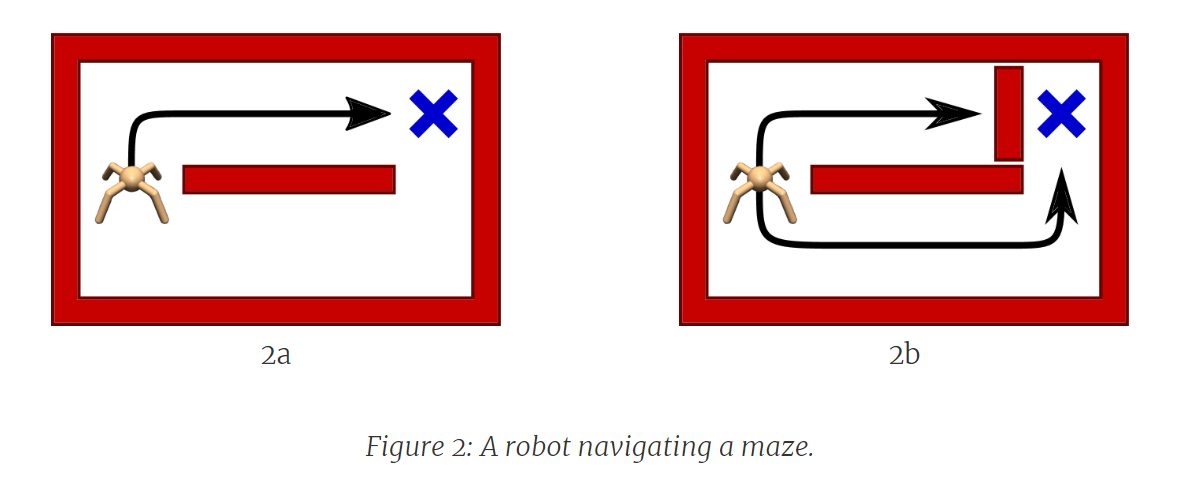
  예를 들어, 다음 Figure에서 거미로봇이 간단한 미로에서 목표(파란색 X)로 가는 길을 찾는 상황을 가정하면, 훈련 시점(Figure 2a)에는 목표로 이어지는 두 개의 통로가 있지만, 에이전트는 약간 더 짧은 위쪽 통로를 통해 해결책을 찾을 가능성이 높으며, 해당 policy을 집중적으로 학습하게 됩니다. (Figure 3a)

  [참고자료 3]의 과대평가(overestimation) 문제 및 Double Q-learning 등에 대한 내용 참고

  

  *출처: Learning Diverse Skills via Maximum Entropy Deep Reinforcement Learning

  그러나 현실세계에서 상단 통로를 벽으로 막는 환경 변화(Figure 2b)가 생기면, 에이전트가 학습한 방법으로는 해결할 수 없을 수 있는데, 이는 학습 동안 에이전트가 전적으로 상단 통로에만 집중했기 때문에, 하단 통로에 대한 학습을 거의 하지 않았기 때문입니다. (Figure 3a)

  따라서 Figure 2b의 새로운 환경에 적응하기 위해서 에이전트는 처음부터 다시 학습해야 합니다.

• 최대 엔트로피 policy과 그 에너지 형태

  RL에서 에이전트는 환경과 상호 작용하면서 현재 상태($s$)를 관찰하고, 행동($a$)을 취하며, 보상($r$)을 받습니다. 에이전트는 확률적 policy($π$)을 사용하여 행동을 선택하고, 에피소드 길이 $T$ 동안 수집한 누적 보상을 최대화하는 최적의 policy을 찾습니다.

  \[\pi^* = \arg\max_\pi \mathbb{E}_\pi \left[\sum_{t=0}^T r_t \right]\]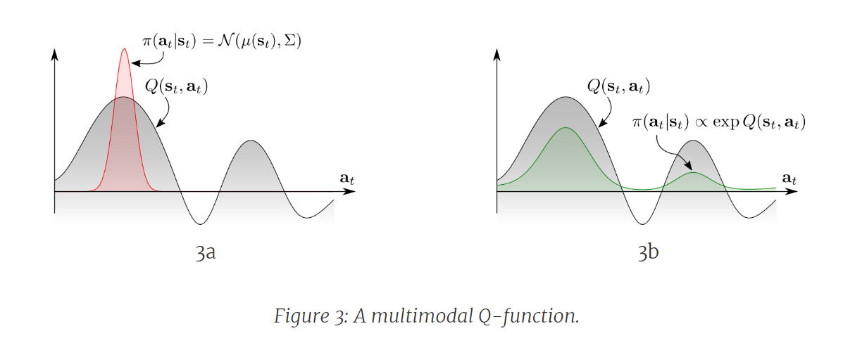
  

  *출처: Learning Diverse Skills via Maximum Entropy Deep Reinforcement Learning

  Q-function,$Q(s,a)$,은 상태 $s$에서 행동 $a$를 취한 후 예상되는 누적 보상으로 정의되는데, Figure 2a의 거미로봇을 사례에서 거미로봇이 초기 상태에 있을 때의 Q-function은 Figure 3a(회색 곡선)에 표시된 두 개의 통로를 나타내는 두 개의 명확한 모드를 가질 수 있습니다. 전통적인 RL 접근 방식은 최대 Q-값에 중심을 둔 단일 모드 policy 분포를 지정하고, 탐색을 위해 인접 행동에 노이즈를 제공합니다. (Figure 3a의 적색 분포) 상단 통로에 대한 탐색이 편향되어 있기 때문에 에이전트는 그곳에서 policy을 정제하고 하단 통로를 완전히 무시하게 됩니다.

• 최대 엔트로피 목적함수로 소프트 벨만 방정식과 소프트 Q-learning

  위와 같은 현상을 방지하기 위해 소프트 벨만 방정식을 사용한 소프트 Q-learning을 사용하며, 최대 엔트로피 목적을 달성하기 위해 소프트 벨만 방정식을 사용하면 다음과 같이 변형할 수 있습니다.

  \[Q(s_t, a_t) = \mathbb{E}[r_t + \gamma \text{softmax}_a Q(s_{t+1}, a)]\]

  위 식에서,

  \[\text{softmax}_a f(a) := \log \int \exp f(a) \, da\]

  소프트 벨만 방정식은 엔트로피가 증가된 보상 함수에 대한 최적 Q-function에 대해 유효함을 볼 수 있습니다. (Ziebart 2010)

  이는 전통적인 벨만 방정식과 유사하지만, 행동에 대한 (하드) 맥스 대신 소프트맥스를 사용합니다. 하드 버전처럼 소프트 벨만 방정식도 마찬가지로 수축성을 갖기때문에 동적 프로그래밍(DP) 또는 모델-프리 TD 학습을 사용하여 표 형태의 상태 및 행동 공간에서 Q-function을 해결할 수 있는 것으로 알려져있습니다. (Ziebart, 2008; Rawlik, 2012; Fox, 2016)

  *출처: Learning Diverse Skills via Maximum Entropy Deep Reinforcement Learning

• [참고자료 6] Step 4 다시 이해해보기

  포스트에서 소프트 벨만 방정식에 대한 컨셉을 이해했으므로, 위에서 논의된 소프트 Q-learning의 소프트 벨만 방정식을 적용하여 최대 엔트로피 목적을 달성하는 방법에 대해 다시 한 번 살펴봅니다. 이 내용은 [참고자료 6] Step 4와 동일합니다.

  • 소프트 벨만 방정식의 적용과 최대 엔트로피 목적의 달성

    소프트 벨만 방정식은 최대 엔트로피 강화학습의 핵심 구성 요소로 다음과 같이 정의됩니다.

    \[Q(s_t, a_t) = \mathbb{E}[r_t + \gamma \text{softmax}_a Q(s_{t+1}, a)]\]

    수식에서 $\text{softmax}_a$는 각 행동의 값을 지수 함수로 변환하고 이를 모두 합한 값의 로그를 취하는 함수입니다. 이 함수는 다음과 같이 표현됩니다.

    \[\text{softmax}_a f(a) := \log \int \exp f(a) \, da\]

    이 소프트맥스 함수는 각 행동의 Q-값을 부드럽게 최대화하여 행동 선택의 확률분포를 더 넓게 만들어 다양한 행동을 탐색할 수 있게 합니다.

    즉, 전통적인 벨만 방정식에서는 최대 Q-값을 선택하는 ‘(하드) 맥스’ 방식^{[참고자료 3]}을 사용하지만, 소프트 벨만 방정식은 ‘소프트맥스’를 사용합니다.

• 최대 엔트로피 목적함수와 최적 policy의 도출 재조명

  최대 엔트로피 강화학습(Maximum Entropy Reinforcement Learning)의 개념을 사용하여 policy $\pi(u_t | x_t)$를 정의합니다.

  최대 엔트로피 목적을 달성하기 위해, 앞서 설명된 소프트 벨만 방정식을 사용하여 다음과 같이 최적 policy을 도출할 수 있습니다. ($u_t$ == 시간 $t$에서의 행동(action), $x_t$ == 시간 $t$에서의 상태(state))

  \[\pi(u_t \\| x_t) \propto \exp\left(\text{Q^{soft}_\pi(x_t, u_t)}{\alpha}\right)\]
  • 파라미터
    • $\pi(u_t | x_t)$ : 시간 $t$에서 상태 $x_t$가 주어졌을 때 행동 $u_t$를 선택할 조건부 확률
    • $Q^{soft}_\pi(x_t, u_t)$ : 소프트 Q-함수로, 주어진 policy $\pi$ 하에서 상태 $x_t$와 행동 $u_t$의 예상 보상을 조정된 엔트로피 값으로 계산
    • $\alpha$ : 온도 파라미터(temperature parameter)로, 행동 선택의 확률적인 성격을 조절함. ($\alpha$가 크면 행동 선택은 더 균등해지고, 작으면 최적의 행동을 더 강하게 선택)

앞에서 설명한 바와 같이 최대 엔트로피 강화학습은 단순히 최대 보상만을 추구하는 것이 아니라, 선택 가능한 여러 행동들 중에서도 엔트로피를 최대화하여 다양한 행동을 탐색하게 함으로써 에이전트(위 Figure의 거미로봇)가 보다 유연하고 적응력 있게 환경 변화에 대응하도록 해 예측 불가능한 환경에서 에이전트의 성능을 향상시키는 것을 목적으로 합니다.

수식에서 $\propto$는 policy \(\pi(u_t \\| x_t)\)는 \(\exp\left(\text{Q^{soft}_\pi(x_t, u_t)}{\alpha}\right)\)에 비례하는 확률로 $u_t$를 선택한다는 것을 의미하며, \(Q^{soft}_\pi\)가 높은 행동은 높은 확률로 선택되지만, 모든 가능한 행동들이 어느 정도의 확률로 탐색이 될 수 있음을 의미합니다. 이는 확률적 policy(stochastic policy)의 특징이기도 합니다.

1 INTRODUCTION

As large pretrained models have become increasingly performant, the problem of aligning them with human preferences have risen to the forefront of research. This alignment is especially difficult when larger datasets inevitably include suboptimal behaviors. Reinforcement learning from human feedback (RLHF) has emerged as a popular solution to this problem. Using human preferences, RLHF techniques discriminate between desirable and undesirable behaviors with the goal of refining a learned policy. This paradigm has shown promising results when applied to fine-tuning large language models (LLMs) (Ouyang et al., 2022), improving image generation models (Lee et al., 2023), and adapting robot policies (Christiano et al., 2017) – all from suboptimal data. For most RLHF algorithms, this process includes two phases. First, a reward model is trained from collected user preference data. And second, that reward model is optimized by an off-the-shelf reinforcement learning (RL) algorithm.

Unfortunately, this two-phase paradigm is founded on a flawed assumption. Algorithms that learn reward models from preference data require that human preferences are distributed according to the discounted sum of rewards or partial return of each behavior segment. However, recent work (Knox et al., 2022) calls this into question, positing that humans instead provide preferences based on the regret of each behavior under the optimal policy of the expert’s reward function. Intuitively, a human’s judgement is likely based on optimality, instead of which states and actions have higher quantity for reward. As a result, the correct quantity to learn from feedback might not be the reward, but instead the optimal advantage function or, in other words, the negated regret.

In their second phase, two-phase RLHF algorithms optimize the reward function learned from the first phase with RL. In practice, RL algorithms suffer from a suite of optimization challenges stemming from temporal credit assignment, such as the high-variance of policy gradients (Marbach & Tsitsiklis, 2003) or instability of approximate dynamic programming (Van Hasselt et al., 2018). Thus, past works limit their scope to circumvent these issues. For instance, RLHF techniques for LLMs assume a contextual bandit formulation (Ouyang et al., 2022), where the policy receives a single reward value in response to a given query to the user. While this reduces the need for long-horizon credit assignment, and consequently the high variance of policy gradients, in reality user interactions with LLMs are multi-step and sequential, violating the single-step bandit assumption. As another example, RLHF has been applied to low-dimensional state-based robotics problems (Christiano et al., 2017; Sikchi et al., 2023a), a setting where approximate dynamic programming excels, but not yet scaled to more realistic high-dimensional continuous control domains with image inputs. Broadly, RLHF methods not only incorrectly assume that the reward function alone drives human preferences, but also require mitigating the optimization challenges of RL by making restrictive assumptions about the sequential nature of problems or dimensionality.

In this work, we introduce a new family of RLHF methods that use a regret-based model of preferences, instead of the commonly accepted partial return model that only considers the sum of rewards. Unlike the partial return model, the regret-based model directly provides information about the optimal policy. A fortunate outcome of this is that it completely eliminates the need for RL, allowing us to solve RLHF problems in the general MDP framework with high-dimensional state and action spaces. Our key insight is to combine the regret-based preference framework with the principle of Maximum Entropy (MaxEnt), resulting in a bijection between advantage functions and policies. By exchanging optimization over advantages for optimization over policies, we are able to derive a purely supervised learning objective whose optimum is the optimal policy under the expert’s reward. We refer to our approach as Contrastive Preference Learning due to its resemblance with commonly accepted contrastive learning objectives.

CPL has three key benefits over prior work. First, CPL can scale as well as supervised learning because it uses only supervised objectives to match the optimal advantage without any policy gradients or dynamic programming. Second, CPL is fully off-policy, enabling effectively using any offline suboptimal data source. Finally, CPL can be applied to arbitrary Markov Decision Processes (MDPs), allowing for learning from preference queries over sequential data. To our knowledge, no prior methods for RLHF simultaneously fulfill all three of these tenants. To demonstrate CPL’s adherence to the three aforementioned tenants, we show its effectiveness on sequential decision making problems with sub-optimal and high-dimensional off-policy data. Notably, we show that CPL can effectively use the same RLHF fine tuning procedure as dialog models to learn temporally extended manipulation policies in the MetaWorld Benchmark. Specifically, we pretrain policies using supervised learning from high-dimensional image observations, before fine tuning them with preferences. Without dynamic programming or policy gradients, CPL is able to match the performance of prior RL based methods. At the same time, it is 1.6× faster and four times as parameter efficient. When using denser preference data, CPL is able to surpass the performance of RL baselines on 5 out of 6 tasks.

2 PRELIMINARIES

We consider the general reinforcement learning from human feedback (RLHF) problem within a reward-free MDP \(M/r = (S, A, p, \gamma)\) with state space \(S\), action space \(A\), transition dynamics \(p(s_{t+1} \mid s_t, a_t)\), and discount factor \(\gamma\). We assume all states are reachable by some policy. The goal of RLHF is to learn a policy \(\pi(a \mid s)\) that maximizes an expert user’s reward function \(r_E(s, a)\). However, since the reward function is not given in an MDP \(/r\), it must be inferred from the expert’s preferences. Typically, a user preference orders two behavior segments.

Figure 1: While most RLHF algorithms use a two-phase reward learning, then RL approach, CPL directly learns a policy using a contrastive objective. This is enabled by the regret preference model.

3 CONTRASTIVE PREFERENCE LEARNING

Though recent work has shown that human preferences are better modeled by the optimal advantage function or regret, most existing RLHF algorithms assume otherwise. By learning a reward function with a mistaken model of preference and then applying RL, traditional RLHF approaches incur a vast, unnecessary computational expense (Knox et al., 2023). Our aim is to derive simple and scalable RLHF algorithms that are purpose-built for the more accurate regret model of human preferences.

Modeling human preferences with regret is not new, but past work suffers from a number of shortcomings. Specifically, existing algorithms using the regret preference model are brittle, as they rely on estimating gradients with respect to a moving reward function, which thus far has only been approximated by computing successor features and assuming a correct linear or tabular representation of the expert reward function \(r_E\) (Knox et al., 2022; 2023). Consequently, these algorithms appear unsuitable for complex scenarios beyond the simplistic grid world environments in which they have been tested.

The key idea of our approach is simple: we recognize that the advantage function, used in regret preference model, can easily be replaced with the log-probability of the policy when using the maximum entropy reinforcement learning framework. The benefit of this simple substitution is however immense. Using the log-probability of the policy circumvents the need to learn the advantage function or grapple with optimization challenges associated with RL-like algorithms. In sum, this enables us to not only embrace a more closely aligned regret preference model, but also to exclusively rely on supervised learning when learning from human feedback.

In this section, we first derive the CPL objective and show that it converges to the optimal policy for \(r_E\) with unbounded data. Then, we draw connections between CPL and other supervised-learning approaches. Finally, we provide recipes for using CPL in practice. Our algorithms are the first examples of a new class of methods for sequential decision making problems which directly learn a policy from regret based preferences without RL, making them far more efficient.

3.1 FROM OPTIMAL ADVANTAGE TO OPTIMAL POLICY

Under the regret preference model, our preference dataset \(D_{\text{pref}}\) contains information about the optimal advantage function \(A^*(s, a)\), which can intuitively be seen as a measure of how much worse a given action \(a\) is than an action generated by the optimal policy at state \(s\). Therefore, actions that maximize the optimal advantage are by definition optimal actions and learning the optimal advantage function from preferences should intuitively allow us to extract the optimal policy.

Naive approach. When presented with \(D_{\text{pref}}\), one might naively follow the standard RLHF reward modeling recipe, but with advantages. This would equate to optimizing a parameterized advantage \(A_{\theta}\) to maximize the log likelihood of \(D_{\text{pref}}\) given the preference model in Eq. (2), or \(\mathbb{E}[( ext^+, \sigma^-) \sim D_{\text{pref}}] [\log P_{A_{\theta}} [\sigma^+ \succ \sigma^-]]\), where \(P_{A_{\theta}}\) is the preference model induced by the \(\max A_{\theta}\) learned advantage function. Once an advantage function that aligns with the preference data is learned, it could be distilled into a parameterized policy. At first glance, it seems like this simple two-step approach could be used to recover the optimal policy from preference data. However, it turns out that learning a Bellman-consistent advantage function is non-trivial in both standard and MaxEnt RL, making learning a valid intermediate advantage function not only unnecessary, but also harder in practice.

Eliminating the need to learn advantage. In maximum entropy RL, Ziebart (2010) has shown that the following relationship between the optimal advantage function and optimal policy holds: \(\int e^{A^*(s,a)/\alpha} da = 1\). This means that in order for a learned advantage function to be optimal, it must be normalized, that is \(\int A e^{A^*(s,a)/\alpha} da = 1\). Enforcing this constraint is intractable, particularly in continuous spaces with large neural networks, making naively learning \(A_{\theta}\) via maximum likelihood estimation difficult.

However, one might instead notice that the above equation establishes a bijection between the reward \(r\) and the policy \(\pi^*\), namely that the optimal advantage function is proportional to the optimal policy’s log-likelihood:

This means that instead of learning the optimal advantage function, we can directly learn the optimal policy.

Given preferences are distributed according to the optimal advantage function for the expert reward function \(r_E\), we can write the preference model in terms of the optimal policy \(\pi^*\) by substituting Eq. (3) into Eq. (2) as follows,

Thus, the maximum entropy framework has led to a model of human preferences that is solely in terms of the optimal policy \(\pi^*\). Using this equivalent form of the advantage-based preference model, we can directly optimize a learned policy \(\pi_{\theta}\) to match the preference model via maximum likelihood with the following convex objective:

Assuming sufficient representation power, at convergence \(\pi_{\theta}\) will perfectly model the user’s preferences, and thus exactly recover \(\pi^*\) under the advantage-based preference model given an unbounded amount of preference data. Specifically, in Appendix A, we prove the following Theorem: Theorem 1. Assume an unbounded number of preferences generated from a noisy rational regret-preference model with expert advantage function \(A^*\). CPL recovers the optimal policy \(\pi^*\) corresponding to reward \(r_E\).

This proof relies on the bijection between optimal advantage functions and policies in maximum entropy RL and the fact that the regret preference model is identifiable (Knox et al., 2022), meaning the objective can achieve a loss of zero.

Benefits of directly learning the policy. Directly learning \(\pi\) in this manner has several benefits, both practical and theoretical. Perhaps most obviously, directly learning the policy circumvents the need for learning any other functions, like a reward function or value function. This makes CPL extremely simple in comparison to prior work. When scaling to larger models, only learning the policy reduces both complexity and computational cost. Second, as pointed out by prior works (Christiano et al., 2017; Hejna & Sadigh, 2023), reward learning can be harmed by the invariance of Boltzmann rational preference models (Eq. (2)) to shifts; i.e., adding a constant to each exponent does not change \(P [\sigma^+ \succ \sigma^-]\). In CPL the distributional constraint of the policy \((\pi_{\theta}(a \mid s) \geq 0\) for all \(a\) and \(\int A \pi_{\theta}(a \mid s) da = 1)\) remedies this issue, since adding a constant makes \(\int A \pi_{\theta}(a \mid s) da \neq 1\). This removes the need for any complicated normalization scheme. Finally, per previous arguments, the policy’s distributional constraint guarantees that \(\int A e^{A_{\theta}(s,a)/\alpha} da = 1\). Thus, it can be shown that CPL’s learned implicit advantage function is always the optimal advantage function for some reward function. We call this property, defined below, consistency and prove the following Proposition in Appendix A. Definition 1. An advantage function \(A(s, a)\) is consistent if there exists some reward function \(r(s, a)\) for which \(A\) is the optimal advantage, or \(A(s, a) = A^*_r(s, a)\). Proposition 1. CPL learns a consistent advantage function. The consequences of this are that no matter the amount of preference data used, CPL will always learn the optimal policy for some reward function, and adding additional preference data only improves the implicit estimate of \(r_E\).

Connections to Contrastive Learning. When deriving CPL, we intentionally chose to denote preferred and unpreferred behavior segments by “+” and “-” to highlight the similarities between CPL and contrastive learning approaches. Though some two-phase RLHF approaches have drawn connections between their reward learning phase and contrastive learning (Kang et al., 2023), CPL directly uses a contrastive objective for policy learning. Specifically, Eq. (5) is an instantiation of the Noise Constrastive Estimation objective (Gutmann & Hyvärinen, 2010) where a segment’s score is its discounted sum of log-probabilities under the policy, the positive example being \(\sigma^+\) and the negative \(\sigma^-\). In the appendix we show that when applied to ranking data using a Plackett-Luce Model, CPL recovers the InfoNCE objective from Oord et al. (2018) where the negative examples are all the segments ranked below the positive segment. Effectively, CPL has fully exchanged the reinforcement learning objective for a supervised, representation learning objective while still converging to the optimal policy. As marked success has been achieved applying contrastive learning objectives to large-scale datasets and neural networks (Chen et al., 2020; He et al., 2020; Radford et al., 2021), we expect CPL to scale more performantly than RLHF methods that use traditional RL algorithms.

3.2 PRACTICAL CONSIDERATIONS

The Contrastive Preference Learning framework provides a general loss function for learning policies from advantage-based preferences, from which many algorithms can be derived. In this section, we detail practical considerations for one particular instantiation of the CPL framework which we found to work well in practice. In the appendix, we include several instantiations of CPL for different types of data and conservative regularizers.

CPL with Finite Offline Data. Though CPL converges to the optimal policy with unbounded preference data, in practice we are often interested in learning from finite offline datasets. In this setting, policies that extrapolate too much beyond the support of the dataset perform poorly as they take actions leading to out of distribution states. Like many other preference-based objectives, CPL’s objective is not strictly convex (Appendix A.3). Thus, many policies, even those with a high weight on actions not in the dataset, can achieve the same optima of Eq. (5). We demonstrate this by formulating CPL as a logistic regression problem. Let the policy be represented by a one-dimensional vector \(\pi \in \mathbb{R}^{\\|S \times A\\|}\). The difference between positive and negative segments, \(\sum t (\\|s\\| - t)\) can be re-written as a dot-product between \(\pi\) and a “comparison” vector \(x\), whose values are either \(\gamma^t\), \(-\gamma^t\), or 0 indicating membership to the comparison \(\sigma^+ \succ \sigma^-\). Using the logistic function, \(\text{logistic}(z) = \frac{1}{1 + e^{-z}}\), we re-write the CPL objective in the finite case as

where \(\sigma^+_i,t\) denotes the tth timestep of the preferred segment from the ith comparison in \(D_{\text{pref}}\). We can reason about the set of all policies that yield the same CPL loss by assembling all comparison vectors into a matrix \(X\), where the ith row of \(X\) is the vector \(x_i\) for the ith comparison in the dataset. Any changes to \(\log \pi\) in the null space of \(X\) have no effect on the logits of the logistic function, and consequently no effect on the loss. In practice, \(\\|S \times A\\| \gg n\), making the null space of \(X\) often nontrivial such that there are multiple minimizers of the CPL loss, some of which potentially place a high probability on state-action pairs not in the dataset. In Appendix A.3 we provide constructions of \(X\) where this is true. Next, we show how this problem can be resolved by incorporating regularization into the CPL objective.

Regularization. In finite settings, we want to choose the policy that minimizes the CPL loss function while placing higher likelihood on actions in the dataset. To accomplish this, we modify Eq. (5) with a conservative regularizer that assigns lower loss when the policy has higher likelihood on actions in \(D_{\text{pref}}\), keeping it in-distribution. Though there are many possible choices of regularizers, we use an asymmetric “bias” regularizer adapted from An et al. (2023) as it performed best in our experiments. Within our objective, the bias regularizer down-weights negative segments by \(\lambda \in (0, 1)\) as so:

4 EXPERIMENTS

In this section, we address the following questions about CPL: First, is CPL effective at fine-tuning policies from regret-based preferences? Second, does CPL scale to high-dimensional control problems and larger networks? Finally, what ingredients of CPL are important for attaining high performance? Additional experiments and details are included in the appendix.

Preference Data. We evaluate CPL’s ability to learn policies for general MDPs from sub-optimal off-policy rollout data and preferences. In particular, we consider the training procedure commonly used for large foundation models: supervised learning, followed by fine-tuning with RLHF. To do this, we use six tasks from the simulated MetaWorld robotics benchmark (Yu et al., 2020). First, we train baseline policies until they approximately reach a 50% success rate. Then, we rollout 2500 episodes of length 250 for each suboptimal stochastic policy. We then form synthetic preference datasets Dpref of different sizes by sampling segments of length 64 uniformly from the rollout data. We estimate regret-based preference labels using the Q-function and policy of an oracle Soft Actor-Critic (SAC) (Haarnoja et al., 2018) model trained to 100% success on a combination of the suboptimal rollout and online data. In practice, we consider two main types of preference datasets: dense, where we label comparisons between every sampled segment (effectively ranking all segments), and sparse, where we label only one comparison per segment.

Baseline Methods. We consider three strong baselines. The first baseline is supervised fine-tuning (SFT), where a policy is first trained with BC on all segments in \(D_{\text{pref}}\), then further fine-tuned on only the preferred segments, i.e., all \(\sigma^+\) in \(D_{\text{pref}}\). The second baseline is Preference IQL (P-IQL), which learns a reward function from \(D_{\text{pref}}\) assuming the partial return preference model, then subsequently learns a policy to maximize it with Implicit Q-learning (Kostrikov et al., 2022), a state-of-the-art offline RL algorithm. Though P-IQL was first used with the partial return model, here it uses an approximation of \(A^*_{r_E}\) as its reward function, which as we show in Appendix A’s Corollary 1 preserves the optimal policy. In fact, P-IQL should be even more performant with regret-based labels, since \(A^*_{r_E}\) is a highly shaped potential-based reward function for \(r_E\) (Ng et al., 1999; Knox et al., 2023). Hejna & Sadigh (2023) found that a well-tuned implementation of P-IQL outperformed several recent state-of-the-art preference-based RL methods, so we use their implementation. Finally, to demonstrate CPL’s ability to extrapolate beyond the best performance found in the rollout data, we compare to %BC, where a policy is trained with behavior cloning on the top X% of rollouts according to the ground truth \(r_E\).

4.1 HOW DOES CPL PERFORM?

How does CPL perform with state-based observations? Our main state-based results can be found in rows 1 and 3 of Table 1. When using sparser comparison data (row 3), CPL outperforms prior methods in 5 of 6 environments, often by a substantial margin of over P-IQL, particularly in Button Press, Bin Picking, and Sweep Into environments. When applied to datasets with more dense comparisons, CPL outperforms P-IQL even more (row 1), doing so substantially in all environments. Though the dense-comparison datasets have less state-action coverage, they have substantially more preference comparisons than the sparse comparison datasets. We posit that more comparisons per segment is more beneficial to CPL than to P-IQL because of its contrastive objective – more comparison-rich datasets are likely to have more informative positive-negative pairs that help shape the policy. We find that CPL consitently outperforms %BC, indicating the CPL is indeed exhibiting policy improvement beyond the best behaviors in the dataset.

How does CPL scale to high-dimensional observations? To test how CPL’s supervised objectives scale to high-dimensional continuous control problems, we render the MetaWorld datasets discussed above to 64 × 64 images. We use the network architecture from DrQv2 (Yarats et al., 2022) and the same hyper-parameters as our state-based experiments. We additionally use random shift augmentations, which drastically improve the performance of RL from images (Laskin et al., 2020).

Interestingly, we find that Our image-based results can be found in rows 2 and 4 of Table 1. performance moderately increases for SFT but substantially for P-IQL. We posit that this is because data-augmentation, which is inapplicable in state, plays a key role in improving value representation for P-IQL. Despite this, when learning from denser preference data (row 2), CPL still outperforms P-IQL in 4 of 6 environments and ties on Sweep Into. When learning from sparser comparisons (row 4), CPL and P-IQL perform comparably on most tasks, even though CPL is drastically simpler than P-IQL. Again, the gap in performance between CPL and P-IQL is higher with denser comparison data, underscoring the importance of informative negatives.

Table 1: Success rates (in percent) of all methods across six tasks on the MetaWorld benchmark on different datasets. The leftmost column contains the observation modality (state or image), the number of segments in the dataset, and the means of labeling comparisons (dense or sparse). Dense refers to labeling every possible pairwise comparison and sparse refers to labeling only one comparison for every two segments, e.g., 10k comparisons for 20k segments. We run four seeds for state and three seeds for images. We report the maximum average performance across seeds over an 8-checkpoint, 200 episode evaluation window. Further evaluation details are in the appendix. Bolded values are within 1% of the top-performing method. The bottom section shows oracle performance of %BC with access to ground-truth reward.

These results are only more impressive considering CPL’s significant reduction in complexity. P-IQL must learn a reward function, a Q-function, a value function, and a policy. CPL avoids all of this, and only learns a policy, drastically reducing training time and parameter count. As we can see in Table 2, this means that CPL runs 1.62× faster than P-IQL on images and has less than a quarter of the the parameters. As networks get larger and larger, the performance gain from using CPL would only increase.

Figure 2: Left: Performance when increasing the number of comparisons per segment on Drawer Open state with 5k segments on two seeds. Right: Ablations on CPL’s hyperparameters on Drawer Open from State. The dotted vertical line shows when BC pretraining stops.

Finally, we ablate both of CPL’s hyperparameters – the temperature value \(\alpha\) and bias regularizer \(\lambda\) – for Drawer Open on the right of Fig. 2. While CPL generally performs well with all values, we find that higher performance could have been attained with further hyper-parameter tuning, particularly for \(\lambda\). In Appendix B, we ablate more design decisions, like the choice of conservative regularizer.

5 RELATED WORK

Though RLHF has recently surged in popularity, learning policies from human preferences has been a long-studied problem, referred to as preference-based RL (PbRL).

PbRL methods typically start by learning a reward function, usually from pairwise comparisons, then use an RL algorithm for policy optimization (F¨urnkranz et al., 2012). While Akrour et al. (2012; 2011); Wilson et al. (2012) were some of the first examples of PbRL, more recently several works have shown that, provided thousands of queries or sufficient pretraining, PbRL can train deep neural-network policies for control using comparisons (Christiano et al., 2017; Lee et al., 2021; Ibarz et al., 2018; Brown et al., 2020; Hejna & Sadigh, 2022; Shin & Brown, 2021) or rankings (Brown et al., 2019; Bıyık et al., 2019; Sikchi et al., 2023a). These approaches, however, are generally demonstrated only on low-dimensional state-based control because of the challenges RL faces when scaling to larger inputs and networks (Ota et al., 2021). In the past, removing RL has lead to effective algorithms for goal-conditioned RL from images (Hejna et al.; Eysenbach et al., 2022). CPL does the same but for PbRL. Other works address the problem of selecting feedback (Sadigh et al., 2017; Biyik et al., 2020; Daniel et al., 2015), which we consider complementary because CPL can benefit from higher quality data elicitation.

To scale RLHF, recent approaches for refining LLMs have ignored the temporal component of RL, and instead treated text-generation as a contextual bandits problem (Ziegler et al., 2019). While this approach has proven effective at tasks like (Stiennon et al., 2020; Wu & Hu, 2018), instruction following (Ouyang et al., 2022; Nakano et al., 2021), and even image generation (Lee et al., 2023; Black et al., 2023), it fundamentally ignores the fact that interaction with users is often sequential, spanning multiple turns. Unlike these methods, CPL works with general MDPs. CPL’s unique ability to learn from sequence data with only supervised objectives makes it a prime candidate for scaling to more complex problems. In fact, Direct Preference Optimization (DPO) (Rafailov et al., 2023) recently demonstrated that a supervised objective similar to CPL works better than RL in the contextual bandits setting. We show in Appendix A that DPO can be derived as a special case of CPL in which segments are of length 1 and always start at the same state. This parallels Knox et al. (2023), who show that the common contextual bandit-approach is a special case of the na¨ıve approach from Section 3.

To derive CPL’s objective, we leverage knowledge from works building on the principle of maximum entropy in control (Ziebart et al., 2008; Ziebart, 2010; Haarnoja et al., 2017). The resulting contrastive update directly learns the optimal policy with fully off-policy data. This is unlike many RL-based RLHF algorithms in both langauge (Ziegler et al., 2019) or control (Christiano et al., 2017) which require on policy rollouts and additional learned components that have been shown to increase variance (Hejna & Sadigh, 2023). Similar contrastive learning objectives have shown to be effective for temporal representation learning (Ma et al., 2023), even with preference data (Kang et al., 2023).

6 DISCUSSION

In this work we introduce CPL, a novel framework for RLHF using the regret preference model. Theoretically, we proved that CPL always learns a consistent advantage function and converges to the optimal policy for the expert’s reward function. Practically, we showed that CPL’s supervised objective is able to outperform RL baselines when learning complex manipulation policies from dense preference data while being simpler and 1.6× faster.

Limitations. CPL, like other RLHF approaches, assumes knowledge of the human rater’s temporal discounting (i.e., of the discount factor γ), which in practice would be difficult to communicate. As CPL’s loss function is computed over segments, it requires a substantial amount of GPU memory for large segment sizes. Finally, no model of human behavior is perfect.

Future Directions. Several exciting research directions remain. First is scaling CPL to larger datasets and architectures where we believe its benefits will be more pronounced. One potentially exciting application is LLMs, where CPL enables fine-tuning on multiple steps of turn-based dialogue. To our knowledge, no multi-step preferences dataset currently exists for LLMs. Second, our work only considers offline data generated by suboptimal policies. An online version of CPL could be developed that works with online human feedback, allowing policies to continually improve.