Weight Alignment Tuning Google - WARP**
- Related Project: Private
- Category: Paper Review
- Date: 2024-06-25
WARP: On the Benefits of Weight Averaged Rewarded Policies
- url: https://arxiv.org/abs/2406.16768
- pdf: https://arxiv.org/pdf/2406.16768
- html: https://arxiv.org/html/2406.16768v1
- homepage: https://mixeval.github.io/
- github: https://github.com/Psycoy/MixEval/?tab=readme-ov-file
- abstract: Reinforcement learning from human feedback (RLHF) aligns large language models (LLMs) by encouraging their generations to have high rewards, using a reward model trained on human preferences. To prevent the forgetting of pre-trained knowledge, RLHF usually incorporates a KL regularization; this forces the policy to remain close to its supervised fine-tuned initialization, though it hinders the reward optimization. To tackle the trade-off between KL and reward, in this paper we introduce a novel alignment strategy named Weight Averaged Rewarded Policies (WARP). WARP merges policies in the weight space at three distinct stages. First, it uses the exponential moving average of the policy as a dynamic anchor in the KL regularization. Second, it applies spherical interpolation to merge independently fine-tuned policies into a new enhanced one. Third, it linearly interpolates between this merged model and the initialization, to recover features from pre-training. This procedure is then applied iteratively, with each iteration’s final model used as an advanced initialization for the next, progressively refining the KL-reward Pareto front, achieving superior rewards at fixed KL. Experiments with GEMMA policies validate that WARP improves their quality and alignment, outperforming other open-source LLMs.
Contents
- WARP: On the Benefits of Weight Averaged Rewarded Policies
TL;DR
- LLM을 위한 가중 평균 보상 정책(WARP) 도입
- KL 규제 및 보상 최적화를 통한 성능 및 정렬 향상
- 반복적인 모델 병합 및 KL-보상 파레토 프런트 최적화
| 단계 | 발견된 문제 | 적용된 방법 | 결과 및 개선 사항 |
|---|---|---|---|
| 1단계: 지수 이동 평균(EMA) | KL 규제의 필요성 강조 | 정책 자체의 EMA 사용, 동적 앵커로서 업데이트 | 안정적인 탐색과 효과적인 KL 규제, 자동 KL 완화와 동적 평균 teacher로부터의 추출 혜택 |
| 2단계: 구면 선형 보간(SLERP) | 가중치 유사성으로 인한 한계 | M개의 독립 정책을 SLERP로 병합 | 각각의 독립 정책 강점을 결합하여 높은 보상을 달성, 병합 정책이 더 높은 보상을 유지하면서 KL을 적당히 유지 |
| 3단계: 초기화로의 선형 보간(LITI) | KL과 보상의 최적 균형 필요 | SLERP 병합 정책을 초기화 쪽으로 선형 보간 | 개선된 파레토 프런트 제공, 중간 보간 계수 선택으로 높은 보상과 낮은 KL의 균형 모델 제공 |
| 반복적 WARP | 지속적인 개선과 효율성 증대 필요 | 반복적인 WARP 실행, 각 반복에서 최적화된 파라미터 사용 | 각 반복마다 성능 개선, 최적의 파레토 프런트에 점진적으로 수렴 |
각 단계의 결과는 더 높은 보상을 달성하고, 더 낮은 KL을 유지하며, 최종적으로 더욱 정교하고 효율적인 LLM 정렬을 가능하게 합니다.
WARP (Weight Averaged Rewarded Policies) 주요 발견
관찰 1: 동적 앵커로서의 지수 이동 평균 (EMA)
EMA를 사용하면, 정책이 동적 평균 teacher로부터 증류를 받으며, KL 규제가 자동으로 완화할 수 있다는 것을 언급합니다. 이는 모델이 초기화에서 너무 멀어지지 않으면서도, 필요한 탐색과 학습을 허용하는 균형을 맞추는 데 도움을 줄 수 있음을 의미합니다.
- 학습 전략: 미래 학습에서는 EMA를 활용하여 모델의 안정성을 유지하면서 동시에 새로운 데이터나 상황에 대한 적응력을 향상시키는 전략을 채택해야 합니다.
- 논문 섹션 3.1. Step 1: KL 규제에서 동적 앵커로서의 지수 이동 평균(EMA)
- 지수 이동 평균 앵커를 사용한 정책 훈련은 KL 규제의 자동 열화와 동적 평균 teacher로부터의 증류에서 이득을 얻습니다. 섹션 4.1에서 경험적 증거를 제시합니다.
관찰 2: 독립적으로 보상받은 정책들의 구면 선형 보간 (SLERP)
SLERP를 통해 병합된 정책은 LERP에 비해 높은 보상을 달성하지만 KL이 약간 증가하는 feature를 보이며, 이는 정책들의 강점을 통합하면서도 다양성을 유지할 수 있다는 것을 의미합니다.
-
SLERP 수식
\[\theta_{slerp}(\lambda) = \theta_{init} + \frac{\sin((1-\lambda)\Omega)}{\sin(\Omega)} \delta_1 + \frac{\sin(\lambda\Omega)}{\sin(\Omega)} \delta_2\] - 학습 전략: SLERP를 활용하여 다양한 정책의 장점을 통합하고, 이를 통해 보다 높은 보상과 적절한 KL 수준을 동시에 달성할 수 있는 학습 방법을 개발해야 합니다.
- 논문 섹션 3.2. Step 2: 독립적으로 보상받은 정책들의 구면 선형 보간(SLERP)
- SLERP를 사용하여 정책을 병합하면 LERP와 비교하여 더 높은 보상을 달성하지만, 이는 약간 더 높은 KL을 동반합니다. 이는 보상과 KL 간의 균형을 찾는데 있어 SLERP가 더 효과적임을 보여줍니다. Appendix B와 C.1에서 이론적 및 경험적 차이를 분석합니다.
관찰 3: 선형 보간 (LERP)
LERP는 KL을 효과적으로 줄이지만, 보상에는 큰 영향을 미치지 않으며, 이는 보상과 안정성 간의 균형을 찾는데 LERP가 유용할 수 있음을 의미합니다. LERP는 가중치를 초기화 쪽으로 당기는 경향이 있으며, 특히 태스크 벡터 간 각도가 거의 직각일 때 더욱 두드러지고, 이 접근 방식은 KL을 효과적으로 줄이지만, 그 과정에서 생성 가능성의 다양성을 제한할 수 있으므로 보상의 최대화에는 그리 효과적이지 않은 것으로 확인했다고 합니다.
-
LERP 수식
\[\theta_{lerp}(\lambda) = \theta_{init} + \lambda (\theta_1 - \theta_{init}) + (1 - \lambda) (\theta_2 - \theta_{init})\] - 학습 전략: 더 안정적인 모델이 필요한 경우 LERP를 활용하여 KL을 관리하고, 과도한 보상 추구가 모델 성능에 부정적 영향을 미치지 않도록 해야 합니다.
- 논문 섹션: 선형 보간(LERP)은 KL을 감소시키지만, 보상에 미치는 영향은 더 작은 것을 확인했으며, 이 관찰은 경험적으로 섹션 C.1에서 입증합니다. 수식 10과 3에서 이론적 통찰을 제공합니다.
관찰 4: 태스크 벡터(Task Vectors)의 직교성
태스크 벡터가 거의 직각을 이룬다는 것은 독립적인 정책들이 서로 다른 feature을 가지고 있음을 의미합니다. (즉, 정책이 상당히 다른 feature를 가지고 있음을 의미) 이로 인해 SLERP는 각 정책의 독특한 장점을 유지하면서도 효과적으로 통합할 수 있으며, 이런 통합은 보상을 증가시키는 동시에 KL을 적절히 관리하여, 더 우수한 파레토 프론트를 달성할 수 있다고 언급합니다.
- 학습 전략: 서로 다른 feature를 가진 모델들을 통합할 때는 SLERP와 같은 방법을 사용하여 각 모델의 장점을 최대한 활용하고, 모델 간의 충돌을 최소화하는 전략을 적용해야 합니다.
- 논문 섹션: 태스크 벡터(\(\delta\))는 거의 직교 상태(\(\Omega \approx 90^\circ\))를 보이며, 전체 가중치(\(\theta\))는 공선입니다. 섹션 C.2에서 경험적 증거가 제시됩니다.
관찰 5: 초기화 방향의 선형 보간 (LITI)
LITI를 통한 가중치 보간은 기존의 RL 훈련보다 우수한 파레토 프론트를 제공하고, 이는 초기화에서 멀어지지 않도록 하면서도 새로운 행동을 탐색할 수 있는 균형을 제공할 수 있다는 것을 확인합니다.
- 학습 전략: 학습 과정에서 초기화에 가깝게 유지하면서도 필요한 경우 새로운 방향으로의 탐색을 허용하는 전략을 사용해야 합니다. 이를 통해 모델은 안정성과 적응성을 동시에 유지할 수 있습니다.
- 논문 섹션 3.3. Step 3: 초기화를 향한 가중치 보간은 기본 RL 정련 동안 드러난 것보다 우수한 파레토 프론트를 드러냅니다. 섹션 4.3에서 경험적 증거와 이론적 통찰을 제공하며, 이는 파레토 최적화에서 LITI는 고보상을 유지하면서 KL을 감소시키는 데 중요한 역할을 합니다.
관찰 6: 반복적 WARP
반복적인 WARP 적용은 결과를 지속적으로 개선하고 최적의 파레토 프론트에 도달할 수 있게하며, 이는 모델의 지속적인 발전가능성을 보여준다고 언급합니다.
- 학습 전략: 모델을 반복적으로 훈련시키고 각 단계에서 얻은 최적화를 다음 단계의 초기화로 사용하여 지속적으로 모델을 발전시키는 전략을 채택해야 합니다. 이 과정에서 적절한 학습률과 정규화 기법을 조정하여 모델의 과적합을 방지하고, 전체적인 성능을 극대화해야 합니다.
- 논문 섹션: WARP를 반복 적용하면 결과가 개선되어 최적의 파레토 프론트에 수렴한다고 하며, 섹션 4.4와 4.5에서 경험적 증거를 제공합니다. 반복적인 접근 방식은 최초의 초기화를 개선하고, 각 반복에서 얻은 최종 가중치를 다음 반복의 개선된 초기화로 사용합니다.
1. 서론
LLM은 언어, 수학, 코딩 등 복잡한 작업을 수행하는 데 놀라운 능력을 보여줍니다. 이런 능력은 다음 토큰 예측을 통한 사전 훈련에서 비롯되며, 지도 학습(Supervised learning)을 통해 세밀하게 조정됩니다. 하지만, LLM이 휴먼의 가치와 일치하는 방향으로 발전함에 따라 안전한 배포를 보장하는 것이 점점 중요해집니다. 이를 위해, 휴먼의 피드백에서 학습하는 강화 학습(RLHF)이 주요 전략으로 부상하고 있습니다. RLHF는 휴먼의 선호도에 따라 보상 모델을 학습한 후, 예측된 보상을 최대화하도록 LLM을 최적화합니다. 그러나 RLHF는 한정된 튜닝 범위와 보상 모델의 불완전함으로 인해 여러 챌린지를 내포하고 있습니다.
2. 배경
LLM은 트랜스포머 기반으로, 파라미터 $\theta$를 사용하여 모델화됩니다. 이 파라미터들은 다음 토큰 예측을 통한 사전 훈련, 지도 학습을 통한 파인튜닝, 그리고 최종적으로 휴먼의 선호를 반영한 보상 모델을 최적화하는 RLHF 단계를 거칩니다. RL 단계에서는 프롬프트 $x$로부터 토큰 시퀀스 $y$를 자동 회귀적으로 생성하는 정책 $\pi_{\theta}(y | x)$를 정의하며, 주된 목표는 데이터셋의 프롬프트에 대해 평균 보상을 최대화하는 것입니다.
\[\arg\max_{\theta} \mathbb{E}_{x \in X} \mathbb{E}_{y \sim \pi_{\theta}(y \\| x)}[r(x, y)]\]KL 대 보상 최적화는 오로지 $r$을 최적화하는 것이 사전 훈련된 일반 능력을 잊게 하고, 보상을 해킹할 수 있는 위험을 내포하며, 생성의 다양성을 줄일 수 있습니다. 이를 완화하기 위해 KL 규제가 도입되어 초기화와의 충실도와 높은 보상 사이의 균형을 이루게 합니다.
\[\arg\max_{\theta} \mathbb{E}_{x \in X} \left[\mathbb{E}_{y \sim \pi_{\theta}(y \\| x)}[r(x, y)] - \beta \text{KL}[\pi_{\theta}(y \\| x) \\\| \pi_{\text{anchor}}(y \\| x)]\right],\]$\theta_{\text{anchor}} \leftarrow \theta_{\text{sft}}$이고, $\beta$는 규제의 강도입니다. 높은 $\beta$ 값은 낮은 KL을 가져오지만, 보상 또한 낮아집니다. REINFORCE 알고리즘은 이런 KL-보상 파레토 최적성을 비교적 잘 달성합니다.
3. 방법
본 논문에서는 가중 평균 보상 정책(Weight Averaged Rewarded Policies, WARP)이라는 새로운 정렬 전략을 도입하였습니다. 이 전략은 LLM의 가중치 공간에서 모델을 병합하여 KL-보상 파레토 프런트를 향상시킵니다. 다음 섹션 3.1에서 3.3에서는 WARP의 세 가지 단계에 걸쳐 다양한 가중 평균(WA) 변형을 적용하는 동기를 설명합니다.
WARP (Weight Averaged Rewarded Policies)
WARP는 세 가지 주요 단계를 통해 LLM의 정렬을 최적화하는 전략입니다.
1단계: 지수 이동 평균(EMA)
이 단계에서는 정책을 지도 학습 모델의 초기화가 아닌, 정책 자체의 지수 이동 평균을 동적으로 업데이트 가능한 앵커로 사용하여 KL을 규제합니다. 이는 안정적인 탐색을 가능하게 하고, 평균 teacher로부터의 추출을 허용합니다.
2단계: 구면 선형 보간(SLERP)
독립적으로 파인튜닝된 정책들을 작업 벡터에 대해 구면 선형 보간을 통해 병합합니다. 이 단계는 각각의 독립 정책의 강점을 결합하여 보상이 높은 병합된 모델을 생성합니다.
3단계: 초기화로의 선형 보간(LITI)
SLERP로 병합된 정책을 초기화 쪽으로 선형 보간합니다. 이는 단순히 보간 계수 $\eta$를 1에서 0 사이로 조절함으로써 개선된 파레토 프런트를 실행할 수 있게 합니다. 중간값 $\eta$를 선택함으로써, 보상은 높지만 KL은 낮은 균형 잡힌 모델을 제공할 수 있습니다. 이는 WARP의 반복적 실행을 위한 새롭고 개선된 초기화로 사용될 수 있습니다.
3.1. 첫 번째 단계: KL 규제에서 동적 앵커로서의 지수 이동 평균(EMA)
EMA 앵커. KL 규제 방법은 일반적으로 지도 학습 초기화를 정적 앵커로 사용합니다. 그러나 제어 작업에서는 정기적으로 앵커를 업데이트하는 것이 일반적입니다. 이에 착안하여 WARP는 정책의 지수 이동 평균(EMA)을 사용하고, RL 파인튜닝 과정에서 지속적으로 업데이트합니다.
\[\theta_{\text{ema}} \leftarrow (1 - \mu) \cdot \theta_{\text{ema}} + \mu \cdot \theta_{\text{policy}}\]관찰 1 (EMA) 지수 이동 평균 앵커를 사용한 정책은 KL 규제의 자동 완화와 동적 평균 teacher로부터의 추출 혜택을 받습니다. 이는 4.1 절에서 경험적으로 확인됩니다.
3.2. 두 번째 단계: 독립적으로 보상된 정책의 구면 선형 보간(SLERP)
SLERP EMA는 단일 RL과 고정된 컴퓨트 예산에서 도움이 되지만, 단일 파인튜닝을 따라 수집된 가중치의 유사성으로 인한 한계가 있습니다. 이 두 번째 단계에서는 독립적으로 파인튜닝된 $M$개의 가중치를 병합합니다.
\[\text{slerp}(\theta_{\text{init}}, \theta_1, \theta_2, \lambda) = \theta_{\text{init}} + \frac{\sin[(1 - \lambda)\Omega]}{\sin \Omega} \cdot \delta_1 + \frac{\sin[\lambda\Omega]}{\sin \Omega} \cdot \delta_2\]SLERP와 LERP의 이점 비교 SLERP는 각 정책의 능력을 결합하며, 그 차이는 SLERP가 규범을 보존하여 기본 모델보다 높은 보상을 달성한다는 것입니다. 반면, LERP는 더 표준적이며 보상에 덜 영향을 미치지만 KL을 줄이는 이점이 있습니다.
3.3. 세 번째 단계: 초기화 쪽으로의 선형 보간(LITI)
LITI 이전 단계에서 SLERP는 여러 정책을 높은 보상과 약간 높은 KL을 가진 하나의 정책으로 결합합니다. 이 세 번째 단계에서는 병합된 모델을 초기화 쪽으로 선형 보간합니다.
\[\theta_{\eta} \leftarrow (1 - \eta) \cdot \theta_{\text{init}} + \eta \cdot \theta_{\text{slerp}}\]$\eta$ 값을 조정함으로써, 새로 획득한 행동과 SFT 초기화에서의 일반 지식 사이에서 균형을 맞출 수 있습니다. $\eta$ 값이 큰 경우 높은 보상을 제공하지만 높은 KL을 야기합니다.
관찰 5 (LITI) 초기화 쪽으로 가중치를 보간하면 RL 파인튜닝 중에 나타난 것보다 나은 파레토 프런트를 밝혀냅니다. 이는 4.3 절과 Figure 1(b)에서 경험적으로 증명됩니다.
3.4. 반복적 WARP
반복 훈련. 이전에 설명한 모델 병합 전략들은 개선된 파레토 프런트를 설정할 뿐만 아니라, 반복적인 개선을 위한 무대를 마련합니다. 충분한 컴퓨트 예산이 있다면, 이 세 단계를 반복적으로 적용할 수 있습니다.
관찰 6 (반복적 WARP) WARP를 반복적으로 적용하면 결과가 개선되며, 최적의 파레토 프런트에 수렴합니다. 이는 4.4 및 4.5 절에서 경험적으로 입증합니다.
4. 실험: WARP의 이점
설정 Gemma “7B” LLM을 더 나은 대화 에이전트로 파인튜닝하기 위해 KL-규제 보상을 최적화하는 REINFORCE Policy 그래디언트를 사용합니다. 데이터셋 X에는 대화 프롬프트가 포함됩니다. 정책의 독립적인 병합과 초기화 쪽으로의 선형 보간을 통해 KL-보상 파레토 프런트를 개선합니다.
4.1. 첫 번째 단계: KL 규제에서 동적 앵커로서의 지수 이동 평균
Figure 3(a) 및 3(b)에서는 다양한 REINFORCE 변형의 훈련 궤적을 비교하며, KL 규제의 앵커 선택과 𝛽의 강도 변경을 보여줍니다. 제안된 버전은 EMA의 정책으로 𝛽 = 0.1과 EMA 업데이트 속도 𝜇 = 0.1을 사용합니다.
4.2. 두 번째 단계: 독립적으로 보상된 정책의 구면 선형 보간
Figure 3(c)에서는 SLERP를 통해 정책을 보간할 때의 보상 볼록성을 보여줍니다. SLERP는 일관되게 LERP보다 높은 보상을 얻지만, 약간 더 높은 KL을 가집니다.
4.3. 세 번째 단계: 초기화 쪽으로의 선형 보간
Figure 4(a)에서는 𝑇 단계 동안 훈련된 정책을 병합한 후 LITI 절차를 적용합니다. 𝜂을 변화시키면서 다양한 파레토 프런트를 밝혀내며, 긴 파인튜닝은 높은 KL에서도 성능을 개선합니다.
4.4. 반복적 WARP
Figure 4(c)에서는 섹션 3.4에서 설명한 반복 절차를 적용합니다. 각 반복에서 𝑀 = 2 정책을 훈련시키고, SLERP로 병합한 후, LITI로 초기화 쪽으로 보간하며, 매 반복마다 결과값이 개선됨을 확인합니다.
4.5. 비교 및 벤치마크
훈련된 정책을 Mistral [60] 및 Mixtral [61] LLM과 비교하고, 최신 Gemma “7B” 1.1 릴리스와 인기 벤치마크에서 WARP를 비교합니다. WARP는 특히 수학 벤치마크에서 강한 결과를 보여줍니다.
5. 선행 연구
모델 병합 방법에 대한 연구는 최근에 주목을 받고 있습니다. 전통적인 예측 공간의 앙상블과 달리, 깊은 모델들은 가중치 공간에서 병합될 수 있습니다. 이를 가중 평균(WA)으로 통칭하며, 가장 일반적인 방법은 선형 보간(LERP)입니다. LERP는 단일 실행에서 수집된 체크포인트를 균일하게 평균화하거나 지수 이동 평균(EMA)을 사용하여 평균화합니다. 선형 모드 연결성 관찰에 따라 모델 수프 변형은 다양한 파인튜닝에서 선형적으로 보간합니다. 이는 공유된 사전 훈련으로 인해 발산을 제한하며, 사전 훈련이 기울기 업데이트의 명시적인 신뢰 영역을 집행할 필요를 완화시킵니다. 이와 대조적으로, 상대적으로 학계에서 덜 탐구된 구면 선형 보간(SLERP)을 사용합니다.
모델 병합의 이점
WA는 분산을 줄이고, 기억력을 감소시키며, 손실 풍경을 평탄화하여 일반화를 증진시킵니다. 또한, 가중치를 병합함으로써 그 강점을 결합할 수 있어, 다중 작업 설정에서 유용합니다. 특히, WA는 RL 설정에서도 사용되며, 보상 모델을 병합하여 효율성과 강건성을 향상시키는 WARM 등이 있습니다. WARP는 WARM에 대한 응답으로 개발되었으며, 모델 병합이 RLHF에서 정책 학습과 보상 설계의 두 가지 주요 챌린지를 해결할 수 있음을 보여줍니다.
6. 토론
분산 학습과 오픈 소스를 위한 병렬화입니다. WARP는 LLM을 휴먼의 가치와 사회적 규범과 일치시키는 중요한 챌린지를 해결합니다. 정책들이 병렬로 훈련되면, 단일 정책 내에서 강점을 결합할 수 있는 능력이 있습니다. WARP의 분산된 성격은 유연성과 확장성을 제공하며, 작업자 간에 간헐적인 가중치 공유를 가능하게 합니다. WARP는 오픈 소스 공동 훈련을 촉진할 수 있으며, 연방 학습 시나리오에서 리소스를 최적화하고 개인 정보를 보호할 수 있습니다.
이터레이션 증폭
WARP는 이터레이션 증폭과 여러 에이전트의 점진적 협력 원칙을 활용하여 LLM의 정렬을 개선합니다. 모델 병합을 통해 에이전트들이 가중치 공간 내에서만 필수 정보를 유지하면서 의사소통할 수 있습니다. 그런 다음, WARP는 다양한 모델에서의 통찰력과 탐색을 결합하여 자기 증류를 통해 점진적으로 높은 보상을 달성합니다.
7. 결론
Weight Averaged Rewarded Policies (WARP)는 LLM을 정렬하기 위한 새로운 RLHF 전략입니다. WARP는 세 가지 모델 병합 단계를 사용하여 KL-보상 파레토 프런트를 개선하고, 사전 훈련에서 얻은 지식을 보호하며, SOTA 베이스 라인과 비교하여 유리한 결과를 제공합니다. WARP가 안전하고 강력한 AI 시스템에 기여하고 모델 병합의 매력을 더 깊이 탐구하는 데 도움이 되기를 기대합니다.
1 Introduction
LLM alignment. Conversational agents like Gemini [36, 110] and GPT-4 [93], along with their open-weight counterparts like Gemma [129], have demonstrated remarkable abilities in complex tasks including mathematics, coding, and tool use [13]. These capabilities largely emerge from pre- training on next-token prediction [101, 102], subsequently refined through supervised fine-tuning (SFT) [105, 135]. As these LLMs become more powerful, aligning them with human values becomes increasingly crucial to ensure safe deployment [5, 46]. To this end, reinforcement learning from human feedback (RLHF) has become the prominent strategy [20, 122, 145], first learning a reward model (RM) on human preferences, before optimizing the LLM to maximize predicted rewards.
Challenges in RLHF. However, RLHF introduces several unresolved challenges [16]. First, the limited scope of fine-tuning, often restricted to relatively small datasets, can lead to excessive specialization and catastrophic forgetting [31] of the broad and diverse knowledge acquired during pre-training [38, 66, 67, 79]. Such alignment tax [97] can degrade the LLM’s reasoning capabilities and performance on NLP benchmarks [25, 81]. Second, maximizing an imperfect RM presents several issues on its own, as the LLM can learn to exploit loopholes in the RM [21, 98] when it deviates significantly from its initialization [33]. Such reward hacking [7, 120] can produce outputs that are linguistically flawed [77], excessively verbose [119], or sycophantic [99, 116], thereby raising misalignment [90, 128] and safety [5, 46] concerns. Finally, RLHF can reduce the diversity of generations [65], potentially leading to policy collapse [42, 86]. Such loss of diversity limits use in creative or exploratory tasks and can result in the LLM systematically refusing to answer. Overall, achieving high rewards based on an imperfect RM on a selected distribution of prompts is insufficient due to potential reward misspecification and distribution shifts upon deployment.
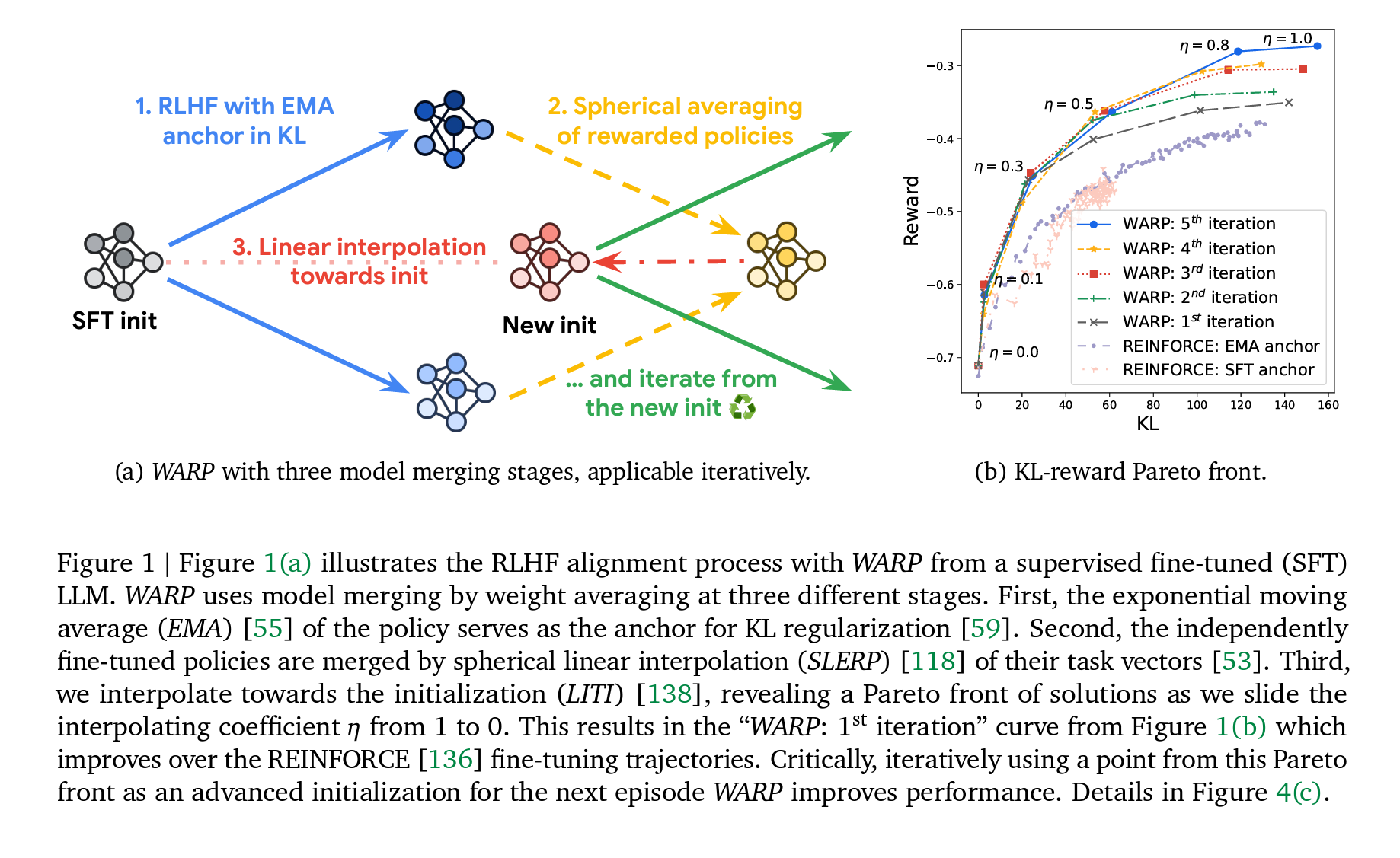
(a) WARP with three model merging stages, applicable iteratively.
(b) KL-reward Pareto front.
Figure 1 Figure 1(a) illustrates the RLHF alignment process with WARP from a supervised fine-tuned (SFT) LLM. WARP uses model merging by weight averaging at three different stages. First, the exponential moving average (EMA) [55] of the policy serves as the anchor for KL regularization [59]. Second, the independently fine-tuned policies are merged by spherical linear interpolation (SLERP) [118] of their task vectors [53]. Third, we interpolate towards the initialization (LITI) [138], revealing a Pareto front of solutions as we slide the interpolating coefficient 𝜂 from 1 to 0. This results in the “WARP: 1st iteration” curve from Figure 1(b) which improves over the REINFORCE [136] fine-tuning trajectories. Critically, iteratively using a point from this Pareto front as an advanced initialization for the next episode WARP improves performance. Details in Figure 4(c).
RL with KL regularization. To address these issues, previous works constrained the reward opti- mization by integrating a Kullback-Leibler (KL) regularization [35, 59], using the SFT initialization as the anchor. As clarified in Section 2, this KL regularization forces the policy to remain close to its initialization [74, 84], mitigating forgetting and reward hacking [33]. However, employing the SFT model as the anchor may lead to reward underfitting: indeed, there is a fundamental tension between reducing KL and maximizing reward. Thus, different policies should be compared in terms of KL-reward Pareto optimality as in Figure 1(b), where the 𝑥-axis is the KL and the 𝑦-axis is the reward as estimated by the RM, with the optimal policies located in the top-left of the plot.
On model merging by weight averaging. To improve the trade-off between KL and reward during RLHF, we leverage the ability to merge LLMs by weight averaging (WA) [131]. WA relies on the linear mode connectivity [30, 89], an empirical observation revealing linear paths of high performance between models fine-tuned from a shared pre-trained initialization. Model merging was shown to improve robustness under distribution shifts [55, 106, 137] by promoting generalization and reducing memorization [108], to combine models’ abilities [52, 53, 109], to reduce forgetting in continual learning [123], to enable collaborative [104] and distributed [27] learning at scale, without computational overheads at inference time. Model merging is increasingly adopted within the open- source community [37, 72], leading to state-of-the-art models in specialized domains [70] but also significant advancements on general-purpose benchmarks [68, 69]. In particular, while WA was initially mostly used for discriminative tasks [137] such as reward modeling [108], it is now becoming popular for generative tasks [4, 111]; its use in KL-constrained RLHF has already shown preliminary successes in a few recent works [39, 81, 83, 88, 92, 109], further elaborated in Section 5.
WARP. In this paper, we propose Weight Averaged Rewarded Policies (WARP), a simple strategy for aligning LLMs, illustrated in Figure 1(a) and detailed in Section 3. WARP is designed to optimize the KL-reward Pareto front of solutions, as demonstrated in Figure 1(b). WARP uses three variants of WA at three different stages of the alignment procedure, for three distinct reasons.
Stage 1: Exponential Moving Average (EMA). During RL fine-tuning, instead of regularizing the policy towards the SFT initialization, WARP uses the policy’s own exponential moving average [100] as a dynamic updatable anchor in the KL. This stage enables stable exploration with distillation from a mean teacher [127] and annealed constraint.
Stage 2: Spherical Linear intERPolation of task vectors (SLERP). Considering 𝑀 policies RL fine-tuned independently with their own EMA anchor, we merge them by spherical linear interpolation [118] of their task vectors [53]. This stage creates a merged model with higher reward by combining the strengths of the 𝑀 individual policies.
Stage 3: Linear Interpolation Towards Initialization (LITI). Considering the merged policy from SLERP, WARP linearly interpolates towards the initialization, akin to WiSE-FT [138]. This stage allows to run through an improved Pareto-front simply by adjusting the interpolating coefficient 𝜂 between 1 (high reward but high KL) and 0 (small KL but small reward). Critically, selecting an intermediate value for 0 < 𝜂 < 1 offers a balanced model that can serve as a new, improved initialization for subsequent iterations of WARP.
Experiments and discussion. In Section 4, we validate the efficacy of WARP for the fine-tuning of Gemma “7B” [129]. Finally, in Section 6, we discuss the connections between WARP, the distributed learning literature [27, 104] and iterated amplification [19], illustrating how WARP embodies their principles to enable scaling post-training, for continuous alignment and improvement of LLMs.
2. Context and notations
RL for LLMs. We consider a transformer [132] LLM \(f(\cdot, \theta)\) parameterized by \(\theta\). Following the foundation model paradigm [12] and the principles of transfer learning [94], those weights are trained via a three-stage procedure: pre-training through next token prediction, supervised fine-tuning resulting in \(\theta_{\text{sft}}\), and ultimately, RLHF [20, 97] to optimize a reward \(r\) as determined by a RM trained to reflect human preferences. In this RL stage, \(\theta\) defines a policy \(\pi_{\theta}(\cdot \\| x)\) by auto-regressively generating token sequences \(y\) from the prompt \(x\). The primary objective is to find weights maximizing the average reward over a dataset of prompts \(X\):
\[\arg\max_{\theta} \mathbb{E}_{x \in X} \mathbb{E}_{y \sim \pi_{\theta}(\cdot \\| x)}[r(x, y)]\]KL vs. reward. Optimizing solely for \(r\) can (i) forget general abilities from pre-training [31] as an alignment tax [81, 97], (ii) hack the reward [7, 120] leading to potential misalignment, or (iii) reduce the diversity of possible generations [65] (confirmed in Appendix F). To mitigate these risks, a KL regularization is usually integrated to balance fidelity to the initialization and high rewards:
\[\arg\max_{\theta} \mathbb{E}_{x \in X} \left[\mathbb{E}_{y \sim \pi_{\theta}(\cdot \\| x)}[r(x, y)] - \beta \text{KL}[\pi_{\theta}(\cdot \\| x) \\\| \pi_{\text{anchor}}(\cdot \\| x)]\right],\]where \(\theta_{\text{anchor}} \leftarrow \theta_{\text{sft}}\) and \(\beta\) is the regularization strength, with high values leading to low KL though also lower reward. The reward function adjusted with this KL is \(r(x, y) - \beta \log \frac{\pi_{\theta}(y \\| x)}{\pi_{\text{anchor}}(y \\| x)}\). Our base RL algorithm is a variant of REINFORCE [136]. This choice follows recent RLHF works [75, 108, 112] and the findings from [2, 80, 126] that, in terms of KL-reward Pareto optimality, REINFORCE performs better than the more complex PPO [114] and also better than various offline algorithms such as DPO [103], IPO [11] or RAFT [26]. Practitioners then typically employ early stopping to select an optimal point on the training trajectory based on their specific use cases.
3. WARP
We introduce a novel alignment strategy named Weight Averaged Rewarded Policies (WARP), illustrated in Figure 1(a) and described in Algorithm 1 below. WARP merges LLMs in the weight space to enhance the KL-reward Pareto front of policies. The following Sections 3.1 to 3.3 describe the motivations behind applying three distinct variants of WA at the three different stages of WARP. In particular, we summarize the key insights as observations, that will be experimentally validated in Section 4 (and in Appendices C and D), and theoretically motivated in Appendix B when possible. Overall, WARP outperforms other RL alignment strategies, without any memory or inference overhead at test time. However, training WARP is costly, requiring multiple RL runs at each iteration: see Section 6 for a detailed discussion on the required compute scaling.
Algorithm 1 WARP for KL-reward Pareto optimal alignment
Input: Weights $\theta_{\text{sft}}$ pre-trained and supervised fine-tuned Reward model $r$, prompt dataset $X$, optimizer Opt
$I$ iterations with $M$ RL runs each for $T$ training steps
$\mu$ EMA update rate, $\eta$ LITI update rate
1: Define $\theta_{\text{init}} \leftarrow \theta_{\text{sft}}$
2: for iteration $i$ from 1 to $I$
do for run $m$ from 1 to $M$
3: $\text{ema} \leftarrow \theta_{\text{init}}$
Define $\theta_m$, $\theta_m$ for step $t$ from 1 to $T$
4: Generate completion $y \sim \pi_{\theta_m}(\cdot \| x)$ for $x \in X$
Compute $r_\beta (y) \leftarrow r(x, y) - \beta \log \frac{\pi_{\theta_m}(y \| x)}{\pi_{\theta_{\text{anchor}}}(y \| x)}$
Update $\theta_m \leftarrow \text{Opt}( ext_m, r_\beta(y) \nabla_{\theta} [\log \pi_{\theta_m}(y \| x)])$
Update $\theta_{\text{ema}} \leftarrow (1 - \mu) \cdot \theta_{\text{ema}} + \mu \cdot \theta_m$
$\text{Run in parallel}$
$\text{KL regularized reward}$
$\text{Policy Gradient}$
$\text{Equation (EMA): update anchor}$
end for
Define $\theta_i$
Update $\theta_{\text{init}} \leftarrow (1 - \eta) \cdot \theta_{\text{init}} + \eta \cdot \theta_i$
$\text{slerp} \leftarrow \text{slerp}( ext_{\text{init}}, {\theta_m}{m=1}^M, \lambda = 1/M)$
$\text{Equation (SLERP): merge $M$ weights}$
$\text{Equation (LITI): interpolate towards init}$
14: end for
Output: KL-reward Pareto front of weights ${(1 - \eta) \cdot \theta{\text{sft}} + \eta \cdot \theta_I}_{0 \leq \eta \leq 1}$
3.1. Stage 1: exponential moving average as a dynamic anchor in KL regularization
EMA anchor. KL-regularized methods typically use the SFT initialization as a static anchor [59, 112], but in RL for control tasks, it is common to regularly update the anchor [1, 113]. In this spirit, WARP uses the policy’s own exponential moving average (EMA) [100], updated throughout the RL fine-tuning process such as, at each training step with $\mu = 0.01$:
\[\theta_{\text{ema}} \leftarrow (1 - \mu) \cdot \theta_{\text{ema}} + \mu \cdot \theta_{\text{policy}}.\](EMA)
Using $\theta_{\text{ema}}$ as the anchor $\theta_{\text{anchor}}$ in Equation (1) provides several benefits, outlined below.
Observation 1 (EMA). Policies trained with an exponential moving average anchor benefit from automatic annealing of the KL regularization and from distillation from a dynamic mean teacher [127]. Empirical evidence in Section 4.1.
3.2. Stage 2: spherical linear interpolation of independently rewarded policies
SLERP. While EMA helps for a single RL and a fixed compute budget, it faces limitations due to the similarity of the weights collected along a single fine-tuning [106]. In this second stage, we merge $M$ weights RL fine-tuned independently (each with their own EMA anchor). This follows model soups from Wortsman et al. [137] and its variants [106, 107] showing that WA improves generalization, and that task vectors [53] (the difference between fine-tuned weights and their initialization) can be arithmetically manipulated by linear interpolation (LERP) [131]. Yet, this time, we use spherical linear interpolation (SLERP) [118], illustrated in Figure 2 and defined below for $M = 2$:
\[\text{slerp}( ext_{\text{init}}, \theta_1, \theta_2, \lambda) = \theta_{\text{init}} + \frac{\sin[(1 - \lambda)\Omega]}{\sin \Omega} \cdot \delta_1 + \frac{\sin[\lambda\Omega]}{\sin \Omega} \cdot \delta_2,\](SLERP)
where $\Omega$ is the angle between the two task vectors \(\delta_1 = \theta_1 - \theta_{\text{init}}\) and \(\delta_2 = \theta_2 - \theta_{\text{init}}\), and $\lambda$ the interpolation coefficient. Critically SLERP is applied layer by layer, each having a different angle. In Appendix B.3 we clarify how SLERP can be used iteratively to merge $M > 2$ models. To enforce diversity across weights, we simply vary the order in which text prompts $x$ are given in each run: this was empirically sufficient, though other diversity strategies could help, e.g., varying the hyperparameters or the reward objectives (as explored in Figure 18(c)).
Benefits from SLERP vs. LERP. Merging task vectors, either with SLERP or LERP, combines their abilities [53]. The difference is that SLERP preserves their norms, reaching higher rewards than the base models; this is summarized in Observation 2. In contrast, and as summarized in Observation 3, the more standard LERP has less impact on reward, but has the advantage of reducing KL; indeed, as shown in Appendix B, LERP tends to pull the merged model towards the initialization, especially as the angle $\Omega$ between task vectors is near-orthogonal (see Observation 3).
3.3. Stage 3: linear interpolation towards initialization
LITI. In the previous stage, SLERP combines multiple policies into one with higher rewards and slightly higher KL. This third stage, inspired by WiSE-FT from Wortsman et al. [138], interpolates from the merged model towards the initialization:
\[\theta_{\eta} \leftarrow (1 - \eta) \cdot \theta_{\text{init}} + \eta \cdot \theta_{\text{slerp}}.\](LITI)
Adjusting the interpolating coefficient $\eta \in [0, 1]$ trades off between some newly acquired behaviors leading to high rewards vs. general knowledge from the SFT initialization. Specifically, large values $\eta \approx 1$ provide high rewards but also high KL, while smaller values $\eta \approx 0$ lean towards smaller rewards and minimal KL. Fortunately, we observe that the reduction in KL is proportionally greater than the reduction in reward when decreasing $\eta$. Then, LITI empirically yields Pareto fronts that are noticeably above the “diagonal”, but also above those revealed during the base RLs.
Observation 5 (LITI). Interpolating weights towards the initialization reveals a better Pareto front than the one revealed during RL fine-tuning. Empirical evidence in Figure 1(b) and Section 4.3, and theoretical insights in Lemmas 4 and 5.
3.4. Iterative WARP
Iterative training. The model merging strategies previously described not only establish an improved Pareto front of solutions, but also set the stage for iterative improvements. Indeed, if the computational budget is sufficient, we can apply those three stages iteratively, using $\theta_{\eta}$ from previous Pareto front (usually with $\eta = 0.3$, choice ablated in Appendix D.3) as the initialization $\theta_{\text{init}}$ for the next iteration, following the model recycling [24, 107] strategies. Then, the entire training procedure is made of multiple iterations, each consisting of those three stages, where the final weight from a given iteration serves as an improved initialization for the next one.
Observation 6 (Iterative WARP). Applying WARP iteratively improves results, converging to an optimal Pareto front. Empirical evidence in Sections 4.4 and 4.5.
4. Experiments: on the benefits of WARP
Setup. We consider the Gemma “7B” [129] LLM, which we seek to fine-tune with RLHF into a better conversational agent. We use REINFORCE [136] policy gradient to optimize the KL-regularized reward. The dataset X contains conversation prompts. We generate on-policy samples with temperature 0.9, batch size of 128, Adam [64] optimizer with learning rate 10−6 and warmup of 100 steps. SLERP is applied independently to the 28 layers. Except when stated otherwise, we train for 𝑇 = 9𝑘 steps, with KL strength 𝛽 = 0.1, EMA update rate 𝜇 = 0.01, merging 𝑀 = 2 policies uniformly 𝜆 = 0.5, and LITI update rate 𝜂 = 0.3; we analyze those values in Appendix D. We rely on a high capacity reward model, the largest available, which prevents the use of an oracle control RM as done in [33, 108].
Summary. In our experiments, we analyze the KL to the SFT policy (reflecting the forgetting of pre-trained knowledge) and the reward (evaluating alignment to the RM). In Section 4.1, we first show the benefits of using an EMA anchor; then in Section 4.2, we show that merging policies trained independently helps. Moreover, in Section 4.3, we show that LITI improves the KL-reward Pareto front; critically, repeating those three WARP stages can iteratively improve performances in Section 4.4. A limitation is that our RM accurately approximates true human preferences only in low KL region, though can be hacked away from the SFT [33]. Therefore, we finally report other metrics in Section 4.5, specifically comparing against open-source baselines such as Mixtral [61], and reporting performances on standard benchmarks such as MMLU [47].
4.1. Stage 1: exponential moving average as a dynamic anchor in KL regularization
In Figures 3(a) and 3(b), we compare the training trajectories of different REINFORCE variants, where the changes lie in the choice of the anchor in the KL regularization and of the hyperparameter 𝛽 controlling its strength. Results are computed every 100 training steps. In our proposed version, the anchor is the EMA of the trained policy with 𝛽 = 0.1 and an EMA update rate 𝜇 = 0.1 (other values are ablated in Figure 15). As the Pareto front for our strategy is above and to the left in Figure 3(b), this confirms the superiority of using such an adaptive anchor. The baseline variants all use the SFT as the anchor, with different values of 𝛽. The lack of regularization (𝛽 = 0.0) leads to very fast optimization of the reward in Figure 3(a), but largely through hacking, as visible by the KL exploding in just a few training steps in Figure 3(b). In contrast, higher values such as 𝛽 = 0.1 fail to optimize the reward as regularization is too strong, causing a quick reward saturation around −0.62 in Figure 3(a). Higher values such as 𝛽 = 0.01 can match our EMA anchor in low KL regime, but saturates around a reward of −0.46. In contrast, as argued in Observation 1, the dynamic EMA anchor progressively moves away from the SFT initialization, causing implicit annealing of the regularization. In conclusion, relaxing the anchor with EMA updates allows the efficient learning of KL-reward Pareto-optimal policies, at any given KL level, for a fixed compute budget. We refer the interested reader to additional experiments in Figure 14 from Appendix D.2 where we compare the trained policies with their online EMA version.
(a) Reward vs. steps.
(b) Reward vs. KL.
(c) SLERP vs. LERP.
Figure 3 EMA and SLERP experiments. We first compare RL runs with different anchors and strengths 𝛽 in the KL regularization. We show their results along training in Figure 3(a), and their KL-reward Pareto fronts in Figure 3(b). We perform evaluation every 100 steps, and train them for 𝑇 = 9𝑘 steps, though we stopped the trainings if they ever reach a KL of 200 (e.g., after 𝑇 = 1𝑘 training steps when 𝛽 = 0.0). Figure 3(c) plots the reward obtained when merging two policies (trained independently after 𝑇 RL steps with their own EMA anchor) with interpolating coefficient 𝜆; highest rewards are with SLERP for 𝜆 = 0.5 and 𝑇 = 9𝑘 steps.
4.2. Stage 2: spherical linear interpolation of independently rewarded policies
In Figure 3(c), we plot 𝜆 → 𝑟 (cid:0)slerp(cid:0)𝜃init, 𝜃1, 𝜃2, 𝜆(cid:1)(cid:1) showing reward convexity when interpolating policies via SLERP, validating Observation 2. This mirrors the linear mode connectivity [30] property across weights fine-tuned from a shared initialization, i.e., the fact that interpolated weights perform better than the initial models (recovered for 𝜆 = 0 or 𝜆 = 1). Moreover, SLERP consistently obtains higher rewards than LERP; yet, this is at slightly higher KL, as further detailed in Appendices B and C.1, where we analyze respectively their theoretical and empirical differences.
4.3. Stage 3: linear interpolation towards initialization
In Figure 4(a), we merge policies trained for 𝑇 steps, and then apply the LITI procedure. Criti- cally, sliding the interpolating coefficient 𝜂 ∈ {0, 0.1, 0.3, 0.5, 0.8, 1.0} reveals various Pareto fronts, consistently above the training trajectories obtained during the two independent RL fine-tunings. Interestingly, longer fine-tunings improve performances, at high KL, but also at lower KL, simply by using a smaller 𝜂 afterwards. Then in Figure 4(b), we report the Pareto fronts when merging up to 𝑀 = 5 weights. We note that all Pareto fronts revealed when applying LITI are consistently above the ones from RL fine-tunings, validating Observation 5. More precisely, best results are achieved by merging an higher number of policies 𝑀, suggesting a promising scaling direction.
4.4. Iterative WARP
In Figure 4(c), we apply the iterative procedure described in Section 3.4. At each of the 𝐼 = 5 iterations we train 𝑀 = 2 policies for 𝑇 steps, with 𝑇 = 9𝑘 for the first iteration, and 𝑇 = 7𝑘 for iterations 2 and 3, and then 𝑇 = 5𝑘 for computational reasons. The LITI curves interpolate towards their own initialization (while Figure 1(b) interpolated towards the SFT initialization, see Appendix D.4 for a comparison). We systematically observe that LITI curves are above the RL training trajectories used to obtain the inits. Results get better at every iteration, validating Observation 6, although with reduced returns after a few iterations.
(a) LITI of SLERP after 𝑇 steps.
(b) LITI of SLERP of 𝑀 weights.
(c) Iterative WARP.
Figure 4 LITI and iterative experiments. Figure 4(a) considers the LITI of the SLERP of 𝑀 = 2 policies after 𝑇 steps with 𝜆 = 0.5, interpolating towards their SFT init as we slide 𝜂, revealing Pareto fronts above the 𝑀 = 2 REINFORCE training trajectories. Then Figure 4(b) plots the LITI of the SLERP of 𝑀 weights with 𝜆 = 1 after 𝑀 𝑇 = 9𝑘 steps: light-colored areas show standard deviations across 5 experiments. The iterative WARP procedure is illustrated in Figure 4(c); we fine-tune 𝑀 = 2 policies with their own EMA as the anchor, merge them with SLERP, interpolate towards their init with LITI, and iteratively leverage the weights obtained with 𝜂 = 0.3 as the new initialization for the next iteration.
4.5. Comparisons and benchmarks
Side by side comparisons. To conclude our experiments, we compare our trained policies against Mistral [60] and Mixtral [61] LLMs. Each policy generates a candidate answer on an held-out collection of prompts, as in the Gemma tech report [129]. Then similarly to Gemini 1.5 [110], we compute side by side preference rates [144] with “much better”, “better” and “slightly better” receiving scores of ±1.5, ±1, and ±0.5 respectively (and ties receiving a score of 0). A positive score represents better policies. The results in Table 1 validate the efficiency of WARP, as our policies are preferred over Mistral variants, and also outperform the two previous Gemma “7B” releases. However, we note that the results stagnate after the 3rd iteration.
Benchmarks. Table 2 compares WARP (3rd iter) and the latest Gemma “7B” 1.1 release [129] on popular benchmarks in the zero-shot setup: MBPP [8] and HumanEval [18] benchmarking coding capabilities, MMLU [47] assessing STEM knowledge, the GSM8K [22] and MATH [48] benchmarks targeting reasoning abilities, and the Big Bench Hard (BBH) [124] benchmark evaluating general capabilities through questions that were deemed difficult for frontier LLMs. WARP has particularly strong results on mathematics benchmarks, suggesting higher analytical capabilities.
Table 2 Benchmark results.
5. Related work
How to merge models. The question of how best to merge models has recently garnered significant attention, driven by the discoveries that deep models can be merged in the weight space [131] instead of in the prediction space, as traditionally done in ensembling [43, 71]. For clarity, we collectively refer to these methods as weight averaging (WA). The most common is LERP, initially used to average checkpoints collected along a single run, uniformly [55, 125] or with an exponential moving average (EMA) [100], notably as a mean teacher [127] for self-supervision [15, 40, 44, 95, 121]. Following the linear mode connectivity [30] observation, the model soups variants [53, 107, 137] linearly interpolate from different fine-tunings; this relies on the shared pre-training, limiting divergence [89] such as models remain in constrained weight regions [41], which also suggests that pre-training mitigates the need to explicitly enforce trust regions in gradient updates [113, 114]. Subsequent works such as TIES merging [140] and DARE [141] reduce interferences in multi-task setups with sparse task vectors [53]. In contrast, we use SLERP, introduced in [118], increasingly popular in the open-source community [37] but relatively underexplored in the academic literature, with limited studies such as [63]. Some tried to align weights trained from scratch [3, 29] or with different architectures [133]; yet, the methods are complex, less robust, and usually require additional training.
Benefits of model merging. WA boosts generalization by reducing variance [106, 137], decreasing memorization [82, 108, 142] and flattening the loss landscape [17]. Additionally, merging weights combines their strengths [53], which helps in multi-task setups [52, 109], to tackle catastrophic forgetting [28, 123] or to provide better initializations [24], as explored in [51, 57, 58] for iterative procedures in classification tasks. In particular, we considered using the geometric insights from Eq. 2 in [58]; yet, as our task vectors are nearly orthogonal Ω ≈ 90◦ (see Appendix C.2), using the update rule 𝜂 → 2 cos Ω failed. WA is now also used in RL setups [34, 73, 91]; for example, WARM [108] 1+cos Ω merges reward models to boost their efficiency, robustness and reliability. Actually, WARP is conceived as a response to WARM, demonstrating that model merging can tackle two key RLHF challenges; policy learning in WARP and reward design in WARM. The most similar works are the following, which also explore how WA can improve policy learning. [92] proposes an iterative approach with the EMA as a new initialization for subsequent iterations. [39] and [88] uses EMA as the reference, but only for direct preference optimization. [109] employs LERP to improve alignment in multi-objective RLHF when dealing with different objectives; similarly, [139] targets multi-task setups with LERP. Finally, [81] and [32] use model merging to reduce the alignment tax, although without incorporating EMA during training, without merging multiple rewarded policies and not iteratively. Critically, none of these works focus on KL as a measure of forgetting, use EMA as the anchor in KL, apply SLERP or use LITI as the initialization for subsequent RL iterations. In contrast, WARP integrates all those elements, collectively leading to an LLM outperforming Mixtral [61].
6. Discussion
Distributed learning for parallelization and open-source. WARP addresses a crucial challenge: aligning LLMs with human values and societal norms, while preserving the capabilities that emerged from pre-training. To this end, we leverage a (perhaps surprising) ability: policies trained in parallel can combine their strengths within a single policy by weight averaging. Then, the distributed nature of WARP makes it flexible and scalable, as it is easily parallelizable by enabling intermittent weight sharing across workers. Actually, iterative WARP shares similarities with DiLoCo [27]: by analogy, the first stage performs inner optimization on multiple workers independently; the second stage merges gradients from different workers; the third stage performs SGD outer optimization with a learning rate equal to 𝜂. More generally, WARP could facilitate open-source [37] collaborative training of policies [104], optimizing resource and supporting privacy in federated learning [85] scenarios; collaborators could train and share their LLMs, while keeping their data and RMs private. In particular, we show in Appendix E that WARP can handle diverse objectives, similarly to [109].
Iterated amplification. WARP improves LLM alignment by leveraging the principles of iterated amplification [19] and progressive collaboration of multiple agents. By analogy, model merging via WA acts as an effective alternative to debate [54], with agents communicating within the weight space instead of the token space, ensuring that only essential information is retained [108]. Then, WARP refines the training signal by combining insights and exploration from diverse models, iteratively achieving higher rewards through self-distillation [127], surpassing the capabilities of any single agent. If this is the way forward, then an iterative safety assessment would be required to detect and mitigate potential risks early, ensuring that the development remains aligned with safety standards.
Scaling alignment. The WARP procedure increases the compute training cost by performing multiple fine-tunings at each iteration. Yet, this should be viewed as “a feature rather than a bug”. Specifically, by preventing memorization and forgetting, we see WARP as a fine-tuning method that can transform additional compute allocated to alignment into enhanced capabilities and safety. This would allow scaling (the traditionally cheap) post-training alignment, in the same way pre-training has been scaled [50]. Critically for large-scale deployment, the acquired knowledge is within a single (merged) model, thus without inference or memory overhead, in contrast to “more agents” approaches [78, 134]. Finally, although WARP improves policy optimization, it is important to recognize that WARP does not address other critical challenges in RLHF [16]: to mitigate the safety risks [5, 45, 46] from misalignment [90, 128], WARP should be part of a broader responsible AI framework.
7. Conclusion
We introduce Weight Averaged Rewarded Policies (WARP), a novel RLHF strategy to align LLMs with three distinct stages of model merging: exponential moving average as a dynamic anchor during RL, spherical interpolation to combine multiple policies rewarded independantly, and interpolation towards the shared initialization. This iterative application of WARP improves the KL-reward Pareto front, aligning the LLMs while protecting the knowledge from pre-training, and compares favorably against state-of-the-art baselines. We hope WARP could contribute to safe and powerful AI systems by scaling alignment, and spur further exploration of the magic behind model merging.